


Analysis of a Digital Comb Filter
In Chapter 1, we extensively analyzed the simplest lowpass
filter,
![]() from a variety of points of view. This
served to introduce many important concepts necessary for
understanding digital filters. In Chapter 2, we analyzed the same
filter using the matlab programming language. This chapter takes
the next step by analyzing a more practical example, the
digital comb filter, from start to finish using the
analytical tools developed in later chapters. Consider this a
``practical motivation'' chapter--i.e., its purpose is to introduce
and illustrate the practical utility of tools for filter analysis
before diving into a systematic development of those tools.
from a variety of points of view. This
served to introduce many important concepts necessary for
understanding digital filters. In Chapter 2, we analyzed the same
filter using the matlab programming language. This chapter takes
the next step by analyzing a more practical example, the
digital comb filter, from start to finish using the
analytical tools developed in later chapters. Consider this a
``practical motivation'' chapter--i.e., its purpose is to introduce
and illustrate the practical utility of tools for filter analysis
before diving into a systematic development of those tools.
Suppose you look up the documentation for a ``comb filter'' in a software package you are using, and you find it described as follows:
    out(n) = input(n) + feedforwardgain * input(n-delay1)
                      - feedbackgain * out(n-delay2)
Does this tell you everything you need to know? Well, it does tell
you exactly what is implemented, but to fully understand it, you must
be able to predict its audible effects on sounds passing
through it. One helpful tool for this purpose is a plot of the
frequency response of the filter. Moreover, if delay1
or delay2 correspond to more than a a few milliseconds of
time delay, you probably want to see its impulse response as
well. In some situations, a pole-zero diagram can give
valuable insights.
As a preview of things to come, we will analyze and evaluate the above example comb filter rather thoroughly. Don't worry about understanding the details at this point--just follow how the analysis goes and try to intuit the results. It will also be good to revisit this chapter later, after studying subsequent chapters, as it provides a concise review of the main topics covered. If you already fully understand the analyses illustrated in this chapter, you might consider skipping ahead to the discussion of specific audio filters in Appendix B, §B.4.
Difference Equation
We first write the comb filter specification in a more ``mathematical'' form as a digital filter difference equation:
where
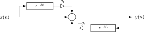
Signal Flow Graph
Figure 3.1 shows the signal flow graph (or system
diagram) for the class of digital filters we are considering (digital
comb filters). The symbol ``![]() '' means a delay of
'' means a delay of ![]() samples (always an integer here). This notation for a pure delay will
make more sense after we derive the filter transfer function in
§3.7.
samples (always an integer here). This notation for a pure delay will
make more sense after we derive the filter transfer function in
§3.7.
 |
Software Implementation in Matlab
In Matlab or Octave, this type of filter can be implemented using the filter function. For example, the following matlab4.1 code computes the output signal y given the input signal x for a specific example comb filter:
g1 = (0.5)^3;        % Some specific coefficients
g2 = (0.9)^5;
B = [1 0 0 g1];      % Feedforward coefficients, M1=3
A = [1 0 0 0 0 g2];  % Feedback coefficients, M2=5
N = 1000;            % Number of signal samples
x = rand(N,1);       % Random test input signal
y = filter(B,A,x);   % Matlab and Octave compatible
The example coefficients,
The matlab filter function carries out the following computation
for each element of the y array:
for
[y1,state] = filter(B,A,x1);       % filter 1st block x1
[y2,state] = filter(B,A,x2,state); % filter 2nd block x2
...
Sample-Level Implementation in Matlab
For completeness, a direct matlab implementation of the built-in
filter function (Eq.![]() (3.3)) is given in Fig.3.2.
While this code is useful for study, it is far slower than the
built-in filter function. As a specific example, filtering
(3.3)) is given in Fig.3.2.
While this code is useful for study, it is far slower than the
built-in filter function. As a specific example, filtering
![]() samples of data using an order 100 filter on a 900MHz Athlon
PC required 0.01 seconds for filter and 10.4 seconds for
filterslow. Thus, filter was over a thousand times
faster than filterslow in this case. The complete test is
given in the following matlab listing:
samples of data using an order 100 filter on a 900MHz Athlon
PC required 0.01 seconds for filter and 10.4 seconds for
filterslow. Thus, filter was over a thousand times
faster than filterslow in this case. The complete test is
given in the following matlab listing:
x = rand(10000,1); % random input signal
B = rand(101,1);   % random coefficients
A = [1;0.001*rand(100,1)]; % random but probably stable
tic; yf=filter(B,A,x); ft=toc
tic; yfs=filterslow(B,A,x); fst=toc
The execution times differ greatly for two reasons:
- recursive feedback cannot be ``vectorized'' in general, and
- built-in functions such as filter are written in C, precompiled, and linked with the main program.
function [y] = filterslow(B,A,x)
% FILTERSLOW: Filter x to produce y = (B/A) x .
%       Equivalent to 'y = filter(B,A,x)' using
%       a slow (but tutorial) method.

NB = length(B);
NA = length(A);
Nx = length(x);

xv = x(:); % ensure column vector

% do the FIR part using vector processing:
v = B(1)*xv;
if NB>1
  for i=2:min(NB,Nx)
    xdelayed = [zeros(i-1,1); xv(1:Nx-i+1)];
    v = v + B(i)*xdelayed;
  end;
end; % fir part done, sitting in v

% The feedback part is intrinsically scalar,
% so this loop is where we spend a lot of time.
y = zeros(length(x),1); % pre-allocate y
ac = - A(2:NA);
for i=1:Nx, % loop over input samples
  t=v(i);   % initialize accumulator
  if NA>1,
    for j=1:NA-1
      if i>j,
        t=t+ac(j)*y(i-j);
      %else y(i-j) = 0
      end;
    end;
  end;
  y(i)=t;
end;

y = reshape(y,size(x)); % in case x was a row vector
|
Software Implementation in C++
Figure 3.3 gives a C++ program for implementing the same filter using the Synthesis Tool Kit (STK). The example writes a sound file containing white-noise followed by filtered-noise from the example filter.
/* main.cpp - filtered white noise example */

#include "Noise.h"  /* Synthesis Tool Kit (STK) class */
#include "Filter.h" /* STK class */
#include "FileWvOut.h"  /* STK class */
#include <cmath>   /* for pow() */
#include <vector>

int main()
{
  Noise *theNoise = new Noise(); // Noise source

  /* Set up the filter */
  StkFloat bCoefficients[5] = {1,0,0,pow(0.5,3)};
  std::vector<StkFloat> b(bCoefficients, bCoefficients+5);
  StkFloat aCoefficients[7] = {1,0,0,0,0,pow(0.9,5)};
  std::vector<StkFloat> a(aCoefficients, aCoefficients+7);
  Filter *theFilter = new Filter;
  theFilter->setNumerator(b);
  theFilter->setDenominator(a);

  FileWvOut output("main");  /* write to main.wav */

  /* Generate one second of white noise */
  StkFloat amp = 0.1; // noise amplitude
  for (long i=0;i<SRATE;i++)   {
    output.tick(amp*theNoise->tick());
  }

  /* Generate filtered noise for comparison */
  for (long i=0;i<SRATE;i++)   {
    output.tick(theFilter->tick(amp*theNoise->tick()));
  }
}
|
Software Implementation in Faust
The Faust language for signal processing is introduced in Appendix K. Figure 3.4 shows a Faust program for implementing our example comb filter. As illustrated in Appendix K, such programs can be compiled to produce LADSPA or VST audio plugins, or a Pure Data (PD) plugin, among others.
/* GUI Controls */
g1  = hslider("feedforward gain", 0.125, 0, 1, 0.01);
g2  = hslider("feedback gain", 0.59049, 0, 1, 0.01);

/* Signal Processing */
process = firpart : + ~ feedback
with {
  firpart(x) = x + g1 * x''';
  feedback(v) = 0 - g2 * v'''';
};
|
Faust's -svg option causes a block-diagram to be written to disk for each Faust expression (as further discussed in Appendix K). The block diagram for our example comb filter is shown in Fig.3.5.
![\includegraphics[width=\twidth]{eps/faustcfbd}](http://www.dsprelated.com/josimages_new/filters/img297.png)
Compiling the Faust code in Fig.3.4 for LADSPA plugin format produces a plugin that can be loaded into ``JACK Rack'' as depicted in Fig.3.6.
![\includegraphics[width=4in]{eps/faustcfjr}](http://www.dsprelated.com/josimages_new/filters/img298.png)
At the risk of belaboring this mini-tour of filter embodiments in common use, Fig.3.7 shows a screenshot of a PD test patch for the PD plugin generated from the Faust code in Fig.3.4.
![\includegraphics[width=3.5in]{eps/faustcfpd}](http://www.dsprelated.com/josimages_new/filters/img299.png) |
By the way, to change the Faust example of Fig.3.4 to include its own driving noise, as in the STK example of Fig.3.3, we need only add the line
import("music.lib");
at the top to define the noise signal (itself only two lines
of Faust code), and change the process definition as follows:
process = noise : firpart : + ~ feedback
In summary, the Faust language provides a compact representation for many digital filters, as well as more general digital signal processing, and it is especially useful for quickly generating real-time implementations in various alternative formats. Appendix K gives a number of examples.
Impulse Response
Figure 3.8 plots the impulse response of the example filter, as computed by the matlab script shown in Fig.3.9. (The plot-related commands are also included for completeness.4.2) The impulse signal consists of a single sample at time 0 having amplitude 1, preceded and followed by zeros (an ideal ``click'' at time 0). Linear, time-invariant filters are fully characterized by their response to this simple signal, as we will show in Chapter 4.
![\includegraphics[width=4in]{eps/eir}](http://www.dsprelated.com/josimages_new/filters/img300.png)
% Example comb filter: g1 = 0.5^3; B = [1 0 0 g1]; % Feedforward coeffs g2 = 0.9^5; A = [1 0 0 0 0 g2]; % Feedback coefficients h = filter(B,A,[1,zeros(1,50)]); % Impulse response % h = impz(B,A,50); % alternative in octave-forge or MSPTB % Matlab-compatible plot: clf; figure(1); stem([0:50],h,'-k'); axis([0 50 -0.8 1.1]); ylabel('Amplitude'); xlabel('Time (samples)'); grid; cmd = 'print -deps ../eps/eir.eps'; disp(cmd); eval(cmd); |
The impulse response of this filter is also easy to compute by hand. Referring to the difference equation

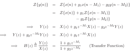
Transfer Function
As we cover in Chapter 6, the transfer function of a digital filter
is defined as
![]() where
where ![]() is the z transform of the input
signal
is the z transform of the input
signal ![]() , and
, and ![]() is the z transform of the output signal
is the z transform of the output signal ![]() . We
may find
. We
may find ![]() from Eq.
from Eq.![]() (3.1) by taking the z transform of both sides
and solving for
(3.1) by taking the z transform of both sides
and solving for ![]() :
:
Some principles of this analysis are as follows:
- The z transform
 is a linear operator which means, by definition,

-
 . That is, the z transform of a signal
  delayed by
  samples,
 , is
, is
 . This is the shift theorem for z transforms, which can
be immediately derived from the definition of the z transform, as shown in
§6.3.
. This is the shift theorem for z transforms, which can
be immediately derived from the definition of the z transform, as shown in
§6.3.
In matlab, difference-equation coefficients are specified as
transfer-function coefficients (vectors B and A in Fig.3.9).
This is why a minus sign is needed in Eq.![]() (3.3).
(3.3).
Ok, so finding the transfer function is not too much work. Now, what
can we do with it? There are two main avenues of analysis from here:
(1) finding the frequency response by setting
![]() , and
(2) factoring the transfer function to find the poles and
zeros of the filter. One also uses the transfer function to generate
different implementation forms such as cascade or parallel
combinations of smaller filters to achieve the same overall filter.
The following sections will illustrate these uses of the transfer
function on the example filter of this chapter.
, and
(2) factoring the transfer function to find the poles and
zeros of the filter. One also uses the transfer function to generate
different implementation forms such as cascade or parallel
combinations of smaller filters to achieve the same overall filter.
The following sections will illustrate these uses of the transfer
function on the example filter of this chapter.
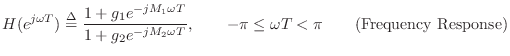
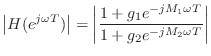
Frequency Response
Given the transfer function ![]() , the frequency response is
obtained by evaluating it on the unit circle in the complex plane,
i.e., by setting
, the frequency response is
obtained by evaluating it on the unit circle in the complex plane,
i.e., by setting
![]() , where
, where ![]() is the sampling interval in
seconds, and
is the sampling interval in
seconds, and ![]() is radian frequency:4.3
is radian frequency:4.3
In the special case
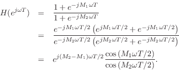
When
![]() , the frequency response is a ratio of cosines in
, the frequency response is a ratio of cosines in
![]() times a linear phase term
times a linear phase term
![]() (which
corresponds to a pure delay of
(which
corresponds to a pure delay of ![]() samples). This special case
gives insight into the behavior of the filter as its coefficients
samples). This special case
gives insight into the behavior of the filter as its coefficients
![]() and
and ![]() approach 1.
approach 1.
When
![]() , the filter degenerates to
, the filter degenerates to ![]() which
corresponds to
which
corresponds to ![]() ; in this case, the delayed input and output
signals cancel each other out. As a check, let's verify this in the
time domain:
; in this case, the delayed input and output
signals cancel each other out. As a check, let's verify this in the
time domain:
![\begin{eqnarray*}
y(n) &=& x(n) + x(n-M) - y(n-M)\\
&=& x(n) + x(n-M) - [x(n-M...
...) - y(n-3M)]\\
&=& x(n) + y(n-3M)\\
&=& \cdots\\
&=& x(n).
\end{eqnarray*}](http://www.dsprelated.com/josimages_new/filters/img331.png)
Amplitude Response
Since the frequency response is a complex-valued function, it has a
magnitude and phase angle for each frequency. The
magnitude of the frequency response is called the amplitude
response (or magnitude frequency response), and it gives the
filter gain at each frequency ![]() .
.
In this example, the amplitude response is
which, for

Figure 3.10a shows a graph of the amplitude response of one case of this filter, obtained by
plotting Eq.![]() (3.5) for
(3.5) for
![]() , and using the
example settings
, and using the
example settings
![]() ,
,
![]() ,
, ![]() , and
, and ![]() .
.
![\includegraphics[width=\twidth]{eps/efr}](http://www.dsprelated.com/josimages_new/filters/img339.png)
Phase Response
The phase of the frequency response is called the phase
response. Like the phase of any complex number, it is given by the
arctangent of the imaginary part of
![]() divided by its
real part, and it specifies the delay of the filter at each
frequency. The phase response is a good way to look at short filter
delays which are not directly perceivable as causing an
``echo''.4.4 For longer delays in audio, it is
usually best to study the filter impulse response, which is
output of the filter when its input is
divided by its
real part, and it specifies the delay of the filter at each
frequency. The phase response is a good way to look at short filter
delays which are not directly perceivable as causing an
``echo''.4.4 For longer delays in audio, it is
usually best to study the filter impulse response, which is
output of the filter when its input is
![]() (an
``impulse''). We will show later that the impulse response is also
given by the inverse
z transform of the filter transfer function (or, equivalently, the inverse
Fourier transform of the filter frequency response).
(an
``impulse''). We will show later that the impulse response is also
given by the inverse
z transform of the filter transfer function (or, equivalently, the inverse
Fourier transform of the filter frequency response).
In this example, the phase response is
freqz(B,A,Nspec).
% efr.m - frequency response computation in Matlab/Octave % Example filter: g1 = 0.5^3; B = [1 0 0 g1]; % Feedforward coeffs g2 = 0.9^5; A = [1 0 0 0 0 g2]; % Feedback coefficients Nfft = 1024; % FFT size Nspec = 1+Nfft/2; % Show only positive frequencies f=[0:Nspec-1]/Nfft; % Frequency axis Xnum = fft(B,Nfft); % Frequency response of FIR part Xden = fft(A,Nfft); % Frequency response, feedback part X = Xnum ./ Xden; % Should check for divide by zero! clf; figure(1); % Matlab-compatible plot plotfr(X(1:Nspec),f);% Plot frequency response cmd = 'print -deps ../eps/efr.eps'; disp(cmd); eval(cmd); |
Pole-Zero Analysis
Since our example transfer function
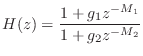

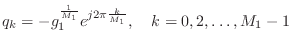
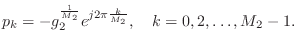
Figure 3.12 gives the pole-zero diagram of the specific example filter
![]() . There are three zeros,
marked by `O' in the figure, and five poles, marked by
`X'. Because of the simple form of digital comb filters, the
zeros (roots of
. There are three zeros,
marked by `O' in the figure, and five poles, marked by
`X'. Because of the simple form of digital comb filters, the
zeros (roots of ![]() ) are located at 0.5 times the three cube
roots of -1 (
) are located at 0.5 times the three cube
roots of -1 (
![]() ), and similarly the poles (roots
of
), and similarly the poles (roots
of ![]() ) are located at 0.9 times the five 5th roots of -1
(
) are located at 0.9 times the five 5th roots of -1
(
![]() ). (Technically, there are also two more
zeros at
). (Technically, there are also two more
zeros at ![]() .) The matlab code for producing this figure is simply
.) The matlab code for producing this figure is simply
[zeros, poles, gain] = tf2zp(B,A); % Matlab or Octave
zplane(zeros,poles); % Matlab Signal Processing Toolbox
                     % or Octave Forge
where B and A are as given in Fig.3.11. The pole-zero plot utility zplane is contained in the Matlab Signal Processing Toolbox, and in the Octave Forge collection. A similar plot is produced by
sys = tf2sys(B,A,1);
pzmap(sys);
where these functions are both in the Matlab Control Toolbox and in Octave. (Octave includes its own control-systems tool-box functions in the base Octave distribution.)
![\includegraphics[width=\twidth]{eps/epz}](http://www.dsprelated.com/josimages_new/filters/img353.png)
Alternative Realizations
For actually implementing the example digital filter, we have only seen the difference equation
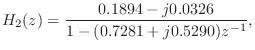
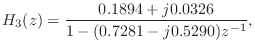
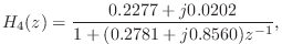
We will now illustrate the computation of a parallel second-order
realization of our example filter
![]() . As discussed above in §3.11, this filter has five
poles and three zeros. We can use the partial fraction
expansion (PFE), described in §6.8, to expand the transfer
function into a sum of five first-order terms:
. As discussed above in §3.11, this filter has five
poles and three zeros. We can use the partial fraction
expansion (PFE), described in §6.8, to expand the transfer
function into a sum of five first-order terms:
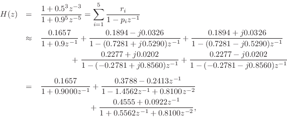
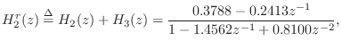
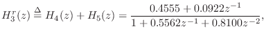
where, in the last step, complex-conjugate one-pole sections are
combined into real second-order sections. Also, numerical values are
given to four decimal places (so `![]() ' is replaced by `
' is replaced by `![]() ' in
the second line). In the following subsections, we will plot the
impulse responses and frequency responses of the first- and
second-order filter sections above.
' in
the second line). In the following subsections, we will plot the
impulse responses and frequency responses of the first- and
second-order filter sections above.
First-Order Parallel Sections
Figure 3.13 shows the impulse response of the real one-pole section
![\includegraphics[width=\twidth]{eps/arir1}](http://www.dsprelated.com/josimages_new/filters/img359.png)
![\includegraphics[width=\twidth]{eps/arfr1}](http://www.dsprelated.com/josimages_new/filters/img360.png)
Figure 3.15 shows the impulse response of the complex one-pole section
![\includegraphics[width=\twidth]{eps/arcir2}](http://www.dsprelated.com/josimages_new/filters/img362.png) |
![\includegraphics[width=\twidth]{eps/arcfr2}](http://www.dsprelated.com/josimages_new/filters/img363.png)
The complex-conjugate section,
![\includegraphics[width=\twidth]{eps/arcir3}](http://www.dsprelated.com/josimages_new/filters/img365.png) |
![\includegraphics[width=\twidth]{eps/arcfr3}](http://www.dsprelated.com/josimages_new/filters/img366.png)
Figure 3.19 shows the impulse response of the complex one-pole section
![\includegraphics[width=\twidth]{eps/arcir4}](http://www.dsprelated.com/josimages_new/filters/img371.png) |
![\includegraphics[width=\twidth]{eps/arcfr4}](http://www.dsprelated.com/josimages_new/filters/img372.png)
Parallel, Real, Second-Order Sections
Figure 3.21 shows the impulse response of the real two-pole section
![\includegraphics[width=\twidth]{eps/arir2}](http://www.dsprelated.com/josimages_new/filters/img375.png) |
![\includegraphics[width=\twidth]{eps/arfr2}](http://www.dsprelated.com/josimages_new/filters/img376.png)
Finally, Fig.3.23 gives the impulse response of the real two-pole section
![\includegraphics[width=\twidth]{eps/arir3}](http://www.dsprelated.com/josimages_new/filters/img378.png) |
![\includegraphics[width=\twidth]{eps/arfr3}](http://www.dsprelated.com/josimages_new/filters/img379.png)
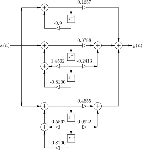
Parallel Second-Order Signal Flow Graph
Figure 3.25 shows the signal flow graph for the implementation of our
example filter using parallel second-order sections (with one
first-order section since the number of poles is odd). This is the
same filter as that shown in Fig.3.1 with ![]() ,
,
![]() ,
, ![]() , and
, and ![]() . The second-order sections are
special cases of the ``biquad'' filter section, which is often
implemented in software (and chip) libraries. Any digital filter can
be implemented as a sum of parallel biquads by finding its transfer
function and computing the partial fraction expansion.
. The second-order sections are
special cases of the ``biquad'' filter section, which is often
implemented in software (and chip) libraries. Any digital filter can
be implemented as a sum of parallel biquads by finding its transfer
function and computing the partial fraction expansion.
 |
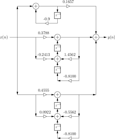 |
The two second-order biquad sections in Fig.3.25 are in so-called ``Direct-Form II'' (DF-II) form. In Chapter 9, a total of four direct-form filter implementations will be discussed, along with some other commonly used implementation structures. In particular, it is explained there why Transposed Direct-Form II (TDF-II) is usually a better choice of implementation structure for IIR filters when numerical dynamic range is limited (as it is in fixed-point ``DSP chips''). Figure 3.26 shows how our example looks using TDF-II biquads in place of the DF-II biquads of Fig.3.25.
Series, Real, Second-Order Sections
Converting the difference equation
![]() to a series bank of real first- and second-order
sections is comparatively easy. In this case, we do not need a full
blown partial fraction expansion. Instead, we need only factor the
numerator and denominator of the transfer function into first- and/or
second-order terms. Since a second-order section can accommodate up
to two poles and two zeros, we must decide how to group pairs of poles
with pairs of zeros. Furthermore, since the series sections can be
implemented in any order, we must choose the section ordering. Both
of these choices are normally driven in practice by numerical
considerations. In fixed-point implementations, the poles and zeros
are grouped such that dynamic range requirements are minimized.
Similarly, the section order is chosen so that the intermediate
signals are well scaled. For example, internal overflow is more likely
if all of the large-gain sections appear before the low-gain sections.
On the other hand, the signal-to-quantization-noise ratio will
deteriorate if all of the low-gain sections are placed before the
higher-gain sections. For further reading on numerical considerations
for digital filter sections, see, e.g., [103].
to a series bank of real first- and second-order
sections is comparatively easy. In this case, we do not need a full
blown partial fraction expansion. Instead, we need only factor the
numerator and denominator of the transfer function into first- and/or
second-order terms. Since a second-order section can accommodate up
to two poles and two zeros, we must decide how to group pairs of poles
with pairs of zeros. Furthermore, since the series sections can be
implemented in any order, we must choose the section ordering. Both
of these choices are normally driven in practice by numerical
considerations. In fixed-point implementations, the poles and zeros
are grouped such that dynamic range requirements are minimized.
Similarly, the section order is chosen so that the intermediate
signals are well scaled. For example, internal overflow is more likely
if all of the large-gain sections appear before the low-gain sections.
On the other hand, the signal-to-quantization-noise ratio will
deteriorate if all of the low-gain sections are placed before the
higher-gain sections. For further reading on numerical considerations
for digital filter sections, see, e.g., [103].
Summary
This chapter has provided an overview of practical digital filter implementation, analysis, transformation, and display. The principal time-domain views were the difference equation and the impulse response. The signal flow graph applies to either time- or frequency-domain signals. The frequency-domain analyses were derived from the z transform of the difference equation, yielding the transfer function, frequency response, amplitude response, phase response, pole-zero analysis, alternate realizations, and related topics. We will take up these topics and more in the following chapters.
In the next chapter, we begin a more systematic presentation of the main concepts of linear systems theory. After that, we will return to practical digital filter analysis, implementation, and (elementary) design.
Next Section:
Linear Time-Invariant Digital Filters
Previous Section:
Matlab Analysis of the Simplest Lowpass Filter


