Analysis of Nonlinear Filters

There is no general theory of nonlinear systems. A nonlinear system with memory can be quite surprising. In particular, it can emit any output signal in response to any input signal. For example, it could replace all music by Beethoven with something by Mozart, etc. That said, many subclasses of nonlinear filters can be successfully analyzed:

A nonlinear, memoryless, time-invariant ``black box'' can be ``mapped out'' by measuring its response to a scaled impulse $\alpha\delta(n)$ at each amplitude $\alpha$ , where $\delta (n)$ denotes the impulse signal ( $[1,0,0,\ldots]$ ).
A memoryless nonlinearity followed by an LTI filter can similarly be characterized by a stack of impulse-responses indexed by amplitude (look up dynamic convolution on the Web).

One often-used tool for nonlinear systems analysis is Volterra series [4]. A Volterra series expansion represents a nonlinear system as a sum of iterated convolutions:

$\displaystyle y = h_0 + h_1 \ast x + ((h_{2,n} \ast x)_n \ast x) + \cdots$

Here

is the input signal,

is the output signal, and the impulse-response replacements

are called Volterra kernels. The special notation $((h_{2,n} \ast x)_n \ast x)$ indicates that the second-order kernel

is fundamentally two-dimensional, meaning that the third term above (the first nonlinear term) is written out explicitly as

$\displaystyle ((h_{2,n} \ast x)_n \ast x) \isdef \sum_{l=0}^\infty\sum_{m=0}^\infty h_2(l,m) x(n-l)x(n-m).$

Similarly, the third-order kernel

is three-dimensional, in general. In principle, every nonlinear system can be represented by its (typically infinite) Volterra series expansion. The method is most successful when the kernels rapidly approach zero as order increases.

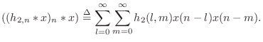
In the special case for which the Volterra expansion reduces to

$\displaystyle y = h_0 + h_1 \ast x + h_2 \ast x \ast x + \cdots\,,$

we have an immediate frequency-domain interpretation in which the output spectrum is expressed as a power series in the input spectrum:

$\displaystyle Y = H_0 + H_1 X + H_2 X^2 + \cdots\,.$

Order a Hardcopy of Introduction to Digital Filters

Previous: A Musical Time-Varying Filter Example
Next: Conclusions

written by Julius Orion Smith III
Julius Smith's background is in electrical engineering (BS Rice 1975, PhD Stanford 1983). He is presently Professor of Music and Associate Professor (by courtesy) of Electrical Engineering at Stanford's Center for Computer Research in Music and Acoustics (CCRMA), teaching courses and pursuing research related to signal processing applied to music and audio systems. See http://ccrma.stanford.edu/~jos/ for details.

Sign in

Search Online Books

Free Online Books

Chapters

Introduction to Digital Filters
Linear Time-Invariant Digital Filters
Analysis of Nonlinear Filters