


The BiQuad Section
The term ``biquad'' is short for ``bi-quadratic'', and is a common name for a two-pole, two-zero digital filter. The transfer function of the biquad can be defined as
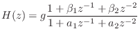
where
As derived in §B.1.3, for real second-order polynomials having
complex roots, it is often convenient to express the polynomial
coefficients in terms of the radius ![]() and angle
and angle ![]() of the
positive-frequency pole. For example, denoting the denominator
polynomial by
of the
positive-frequency pole. For example, denoting the denominator
polynomial by
![]() , we have
, we have
As discussed on page ![]() , a common setting for the zeros when
making a resonator is to place one at
, a common setting for the zeros when
making a resonator is to place one at ![]() (dc) and the other at
(dc) and the other at
![]() (half the sampling rate), i.e.,
(half the sampling rate), i.e., ![]() and
and
![]() in
Eq.
in
Eq.![]() (B.8) above
(B.8) above
![]() .
This zero placement normalizes the peak gain of the resonator if it is
swept using the
.
This zero placement normalizes the peak gain of the resonator if it is
swept using the ![]() parameter.
parameter.
Using the shift theorem for z transforms, the difference equation for the biquad can be written by inspection of the transfer function as
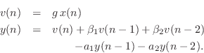
where ![]() denotes the input signal sample at time
denotes the input signal sample at time ![]() , and
, and ![]() is the output signal. This is the form that is typically implemented
in software. It is essentially the direct-form I implementation. (To obtain the official
direct-form I structure, the overall gain
is the output signal. This is the form that is typically implemented
in software. It is essentially the direct-form I implementation. (To obtain the official
direct-form I structure, the overall gain ![]() must be not be pulled
out separately, resulting in feedforward coefficients
must be not be pulled
out separately, resulting in feedforward coefficients
![]() instead. See Chapter 9 for more about
filter implementation forms.)
instead. See Chapter 9 for more about
filter implementation forms.)
Next Section:
Biquad Software Implementations
Previous Section:
Complex Resonator


