When the maximally flat optimality criterion is applied to the general
(analog) squared amplitude response
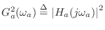 , a surprisingly simple
result is obtained [64]:
, a surprisingly simple
result is obtained [64]:
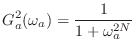 |
(I.1) |
where

is the desired order (number of
poles). This simple result
is obtained when the response is taken to be maximally flat at

as well as
dc (
i.e., when both

and

are maximally flat at dc).
I.1Also, an arbitrary scale factor for

has been set such that
the cut-off frequency (-3dB frequency) is

rad/sec.
The analytic continuation
(§D.2)
of
to the whole
 -plane may be obtained by substituting
 to obtain
The

poles of this expression are simply the
roots of unity when
is odd, and the roots of

when
is even. Half of these
poles

are in the left-half
-plane (
re

) and
thus belong to

(which must be stable). The other half belong
to

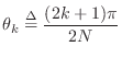
. In summary, the poles of an
th-order Butterworth
lowpass prototype are located in the
-plane at

, where [
64, p. 168]
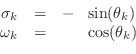 |
(I.2) |
with
for

. These poles may be quickly found graphically
by placing
poles uniformly distributed around the unit circle (in
the
plane, not the

plane--this is not a frequency axis) in
such a way that each complex pole has a complex-conjugate counterpart.
A Butterworth lowpass filter additionally has zeros at  .
Under the bilinear transform
.
Under the bilinear transform
 , these all map to the
point
, these all map to the
point  , which determines the numerator of the digital filter as
 .
.
Given the poles and zeros of the analog prototype, it is straightforward
to convert to digital form by means of the bilinear transformation.
Next Section: Example: Second-Order Butterworth LowpassPrevious Section: Mechanical Equivalent of an Inductor is a Mass