Cyclic Convolution Matrix

An infinite Toeplitz matrix implements, in principle, acyclic convolution (which is what we normally mean when we just say ``convolution''). In practice, the convolution of a signal and an impulse response , in which both and are more than a hundred or so samples long, is typically implemented fastest using FFT convolution (i.e., performing fast convolution using the Fast Fourier Transform (FFT) [84]^F.3). However, the FFT computes cyclic convolution unless sufficient zero padding is used [84]. The matrix representation of cyclic (or ``circular'') convolution is a circulant matrix, e.g.,

$\displaystyle \mathbf{h}= \left[\begin{array}{cccccc} h_0 & 0 & 0 & 0 & h_2 & ... ... h_2 & h_1 & h_0 & 0 \\ [2pt] 0 & 0 & 0 & h_2 & h_1 & h_0 \end{array}\right].$

As in this example, each row of a circulant matrix is obtained from the previous row by a circular right-shift. Circulant matrices are thus always Toeplitz (but not vice versa). Circulant matrices have many interesting properties.^F.4 For example, the eigenvectors of an $N\times N$ circulant matrix are the DFT sinusoids for a length

DFT [84]. Similarly, the eigenvalues may be found by simply taking the DFT of the first row.

The DFT eigenstructure of circulant matrices is directly related to the DFT convolution theorem [84]. The above $6\times 6$ circulant matrix $\mathbf{h}$ , when multiplied times a length 6 vector ${\underline{x}}$ , implements cyclic convolution of ${\underline{x}}$ with $\underline{h}=[h_0,h_1,h_3,0,0,0]$ . Using the DFT to perform the circular convolution can be expressed as

$\displaystyle \underline{y}={\underline{x}}\circledast \underline{h}=$ IDFT $\displaystyle ($ DFT $\displaystyle ({\underline{x}})\cdot$ DFT $\displaystyle (\underline{h})),$

where ` $\circledast$ ' denotes circular convolution. Let $\mathbf{S}$ denote the matrix of sampled DFT sinusoids for a length

DFT: $\mathbf{S}[k,n]\isdeftext e^{j2\pi k n/N}$ . Then $\mathbf{S}^\ast$ is the DFT matrix, where ` $\ast$ ' denotes Hermitian transposition (transposition and complex-conjugation). The DFT of the length-

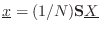
vector ${\underline{x}}$ can be written as $\underline{X}=\mathbf{S}^\ast\,{\underline{x}}$ , and the corresponding inverse DFT is ${\underline{x}}=(1/N)\mathbf{S}\underline{X}$ . The DFT-eigenstructure of circulant matrices provides that a real $N\times N$ circulant matrix $\mathbf{h}$ having top row $\underline{h}^T$ satisfies $\mathbf{h}\mathbf{S}= \mathbf{S}\cdot$ diag $(\underline{H})$ , where $\underline{H}=\mathbf{S}^\ast\,\underline{h}$ is the length

DFT of $\underline{h}$ , and diag $(\underline{H})$ denotes a diagonal matrix with the elements of $\underline{H}$ along the diagonal. Therefore, diag $(\underline{H})=\mathbf{S}^{-1}\mathbf{h}\mathbf{S}=(1/N)\mathbf{S}^\ast\,\mathbf{h}\,\mathbf{S}$ . By the DFT convolution theorem,

$\begin{eqnarray*} \underline{y}=\underline{h}\circledast {\underline{x}} &\Leftr... ...{X}=(1/N)\mathbf{S}^\ast\,\mathbf{h}\,\mathbf{S}\,\underline{X}. \end{eqnarray*}$

Premultiplying by the IDFT matrix $(1/N)\mathbf{S}$ yields

$\displaystyle \underline{y}= (1/N)\mathbf{S}\underline{Y}=(1/N)\mathbf{S}\mathbf{S}^\ast\,\mathbf{h}\,(1/N)\mathbf{S}\underline{X}= \mathbf{h}{\underline{x}}.$

Thus, the DFT convolution theorem holds if and only if the circulant convolution matrix $\mathbf{h}$ has eigenvalues $\underline{H}$ and eigenvectors given by the columns of $\mathbf{S}$ (the DFT sinusoids).

Previous: General LTI Filter Matrix
Next: Inverse Filters

Order a Hardcopy of Introduction to Digital Filters

About the Author: Julius Orion Smith III
Julius Smith's background is in electrical engineering (BS Rice 1975, PhD Stanford 1983). He is presently Professor of Music and Associate Professor (by courtesy) of Electrical Engineering at Stanford's Center for Computer Research in Music and Acoustics (CCRMA), teaching courses and pursuing research related to signal processing applied to music and audio systems. See http://ccrma.stanford.edu/~jos/ for details.

Sign in

Search Online Books

Free Online Books

Chapters

See Also

Introduction to Digital Filters
Matrix Filter Representations
Cyclic Convolution Matrix