


Decay Time is Q Periods
Another well known rule of thumb is that the ![]() of a resonator is the
number of ``periods'' under the exponential decay of its impulse
response. More precisely, we will show that, for
of a resonator is the
number of ``periods'' under the exponential decay of its impulse
response. More precisely, we will show that, for ![]() , the
impulse response decays by the factor
, the
impulse response decays by the factor ![]() in
in ![]() cycles, which
is about 96 percent decay, or -27 dB.
cycles, which
is about 96 percent decay, or -27 dB.
The impulse response corresponding to Eq.![]() (E.8) is found by
inverting the Laplace transform of the transfer function
(E.8) is found by
inverting the Laplace transform of the transfer function ![]() . Since it
is only second order, the solution can be found in many tables of
Laplace transforms. Alternatively, we can break it up into a sum of
first-order terms which are invertible by inspection (possibly after
rederiving the Laplace transform of an exponential decay, which is
very simple). Thus we perform the partial fraction expansion of
Eq.
. Since it
is only second order, the solution can be found in many tables of
Laplace transforms. Alternatively, we can break it up into a sum of
first-order terms which are invertible by inspection (possibly after
rederiving the Laplace transform of an exponential decay, which is
very simple). Thus we perform the partial fraction expansion of
Eq.![]() (E.8) to obtain
(E.8) to obtain
| (E.12) | |||
| (E.13) |
as the respective residues of the poles
The impulse response is thus
Assuming a resonator, ![]() , we have
, we have
![]() , where
, where
![]() (using notation of the
preceding section), and the impulse response reduces to
(using notation of the
preceding section), and the impulse response reduces to
We have shown so far that the impulse response ![]() decays as
decays as
![]() with a sinusoidal radian frequency
with a sinusoidal radian frequency
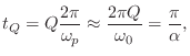
![]() under the exponential envelope. After Q periods at frequency
under the exponential envelope. After Q periods at frequency
![]() , time has advanced to
, time has advanced to
Next Section:
Q as Energy Stored over Energy Dissipated
Previous Section:
Impulse Response


