


Finding the Frequency Response
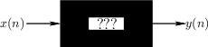
Think of the filter expressed by Eq.![]() (1.1) as a ``black box'' as
depicted in Fig.1.5. We want to know the effect of this black box
on the spectrum of
(1.1) as a ``black box'' as
depicted in Fig.1.5. We want to know the effect of this black box
on the spectrum of ![]() , where
, where ![]() represents the entire
input signal (see §A.1).
represents the entire
input signal (see §A.1).
Sine-Wave Analysis
Suppose we test the filter at each frequency separately. This is
called sine-wave analysis.2.1Fig.1.6 shows an example of
an input-output pair, for the filter of Eq.![]() (1.1), at the
frequency
(1.1), at the
frequency ![]() Hz, where
Hz, where ![]() denotes the sampling rate. (The
continuous-time waveform has been drawn through the samples for
clarity.) Figure 1.6a shows the input signal, and Fig.1.6b
shows the output signal.
denotes the sampling rate. (The
continuous-time waveform has been drawn through the samples for
clarity.) Figure 1.6a shows the input signal, and Fig.1.6b
shows the output signal.
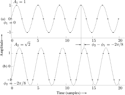 |
The ratio of the peak output amplitude to the peak input amplitude is
the filter gain at this frequency. From Fig.1.6 we find
that the gain is about 1.414 at the frequency ![]() . We may also
say the amplitude response is 1.414 at
. We may also
say the amplitude response is 1.414 at ![]() .
.
The phase of the output signal minus the phase of the input signal is
the phase response of the filter at this
frequency. Figure 1.6 shows that the filter of Eq.![]() (1.1) has a
phase response equal to
(1.1) has a
phase response equal to ![]() (minus one-eighth of a cycle) at the
frequency
(minus one-eighth of a cycle) at the
frequency ![]() .
.
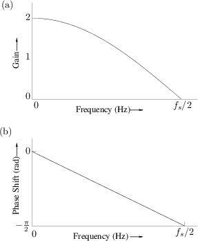
Continuing in this way, we can input a sinusoid at each frequency
(from 0 to ![]() Hz), examine the input and output waveforms as in
Fig.1.6, and record on a graph the peak-amplitude ratio (gain)
and phase shift for each frequency. The resultant pair of plots, shown
in Fig.1.7, is called the frequency response. Note that
Fig.1.6 specifies the middle point of each graph in Fig.1.7.
Hz), examine the input and output waveforms as in
Fig.1.6, and record on a graph the peak-amplitude ratio (gain)
and phase shift for each frequency. The resultant pair of plots, shown
in Fig.1.7, is called the frequency response. Note that
Fig.1.6 specifies the middle point of each graph in Fig.1.7.
Not every black box has a frequency response, however. What good is a pair of graphs such as shown in Fig.1.7 if, for all input sinusoids, the output is 60 Hz hum? What if the output is not even a sinusoid? We will learn in Chapter 4 that the sine-wave analysis procedure for measuring frequency response is meaningful only if the filter is linear and time-invariant (LTI). Linearity means that the output due to a sum of input signals equals the sum of outputs due to each signal alone. Time-invariance means that the filter does not change over time. We will elaborate on these technical terms and their implications later. For now, just remember that LTI filters are guaranteed to produce a sinusoid in response to a sinusoid--and at the same frequency.
Mathematical Sine-Wave Analysis
The above method of finding the frequency response involves physically
measuring the amplitude and phase response for input sinusoids of
every frequency. While this basic idea may be practical for a real
black box at a selected set of frequencies, it is hardly useful for
filter design. Ideally, we wish to arrive at a mathematical
formula for the frequency response of the filter given by
Eq.![]() (1.1). There are several ways of doing this. The first we
consider is exactly analogous to the sine-wave analysis procedure
given above.
(1.1). There are several ways of doing this. The first we
consider is exactly analogous to the sine-wave analysis procedure
given above.
Assuming Eq.![]() (1.1) to be a linear time-invariant filter
specification (which it is), let's take a few points in the frequency
response by analytically ``plugging in'' sinusoids at a few different
frequencies. Two graphs are required to fully represent the frequency
response: the amplitude response (gain versus frequency) and phase
response (phase shift versus frequency).
(1.1) to be a linear time-invariant filter
specification (which it is), let's take a few points in the frequency
response by analytically ``plugging in'' sinusoids at a few different
frequencies. Two graphs are required to fully represent the frequency
response: the amplitude response (gain versus frequency) and phase
response (phase shift versus frequency).
The frequency 0 Hz (often called dc, for direct current)
is always comparatively easy to handle when we analyze a filter. Since
plugging in a sinusoid means setting
![]() ,
by setting
,
by setting ![]() , we obtain
, we obtain
![]() for all
for all ![]() . The input signal, then, is the same number
. The input signal, then, is the same number
![]() over and over again for each sample. It should be clear that
the filter output will be
over and over again for each sample. It should be clear that
the filter output will be
![]() for all
for all ![]() . Thus, the gain at frequency
. Thus, the gain at frequency ![]() is 2, which we get by dividing
is 2, which we get by dividing ![]() , the output amplitude, by
, the output amplitude, by
![]() , the input amplitude.
, the input amplitude.
Phase has no effect at ![]() Hz because it merely shifts a constant
function to the left or right. In cases such as this, where the phase
response may be arbitrarily defined, we choose a value which preserves
continuity. This means we must analyze at frequencies in a
neighborhood of the arbitrary point and take a limit. We will compute
the phase response at dc later, using different techniques. It is
worth noting, however, that at 0 Hz, the phase of every
real2.2 linear
time-invariant system is either 0 or
Hz because it merely shifts a constant
function to the left or right. In cases such as this, where the phase
response may be arbitrarily defined, we choose a value which preserves
continuity. This means we must analyze at frequencies in a
neighborhood of the arbitrary point and take a limit. We will compute
the phase response at dc later, using different techniques. It is
worth noting, however, that at 0 Hz, the phase of every
real2.2 linear
time-invariant system is either 0 or ![]() , with the phase
, with the phase ![]() corresponding to a sign change. The phase of a complex filter
at dc may of course take on any value in
corresponding to a sign change. The phase of a complex filter
at dc may of course take on any value in
![]() .
.
The next easiest frequency to look at is half the sampling rate,
![]() . In this case, using basic trigonometry (see §A.2), we can
simplify the input
. In this case, using basic trigonometry (see §A.2), we can
simplify the input ![]() as follows:
as follows:
 |
|||
 |
|||
| (2.2) |
where the beginning of time was arbitrarily set at
| (2.3) |
The filter of Eq.
If we back off a bit, the above results for the amplitude response are
obvious without any calculations. The filter
![]() is
equivalent (except for a factor of 2) to a simple two-point average,
is
equivalent (except for a factor of 2) to a simple two-point average,
![]() . Averaging adjacent samples in a signal
is intuitively a low-pass filter because at low frequencies the sample
amplitudes change slowly, so that the average of two neighboring
samples is very close to either sample, while at high frequencies the
adjacent samples tend to have opposite sign and to cancel out when
added. The two extremes are frequency 0 Hz, at which the averaging has
no effect, and half the sampling rate
. Averaging adjacent samples in a signal
is intuitively a low-pass filter because at low frequencies the sample
amplitudes change slowly, so that the average of two neighboring
samples is very close to either sample, while at high frequencies the
adjacent samples tend to have opposite sign and to cancel out when
added. The two extremes are frequency 0 Hz, at which the averaging has
no effect, and half the sampling rate ![]() where the samples
alternate in sign and exactly add to 0.
where the samples
alternate in sign and exactly add to 0.
We are beginning to see that Eq.![]() (1.1) may be a low-pass filter
after all, since we found a boost of about 6 dB at the lowest
frequency and a null at the highest frequency. (A gain of 2 may be
expressed in decibels as
(1.1) may be a low-pass filter
after all, since we found a boost of about 6 dB at the lowest
frequency and a null at the highest frequency. (A gain of 2 may be
expressed in decibels as
![]() dB, and a
null or notch is another
term for a gain of 0 at a single frequency.) Of course, we tried only
two out of an infinite number of possible frequencies.
dB, and a
null or notch is another
term for a gain of 0 at a single frequency.) Of course, we tried only
two out of an infinite number of possible frequencies.
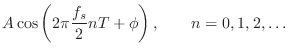
Let's go for broke and plug the general sinusoid into Eq.![]() (1.1),
confident that a table of trigonometry identities will see us through
(after all, this is the simplest filter there is, right?). To set the
input signal to a completely arbitrary sinusoid at amplitude
(1.1),
confident that a table of trigonometry identities will see us through
(after all, this is the simplest filter there is, right?). To set the
input signal to a completely arbitrary sinusoid at amplitude ![]() ,
phase
,
phase ![]() , and frequency
, and frequency ![]() Hz, we let
Hz, we let
![]() . The output is then given by
. The output is then given by
All that remains is to reduce the above expression to a single sinusoid with some frequency-dependent amplitude and phase. We do this first by using standard trigonometric identities [2] in order to avoid introducing complex numbers. Next, a much ``easier'' derivation using complex numbers will be given.
Note that a sum of sinusoids at the same frequency, but possibly different phase and amplitude, can always be expressed as a single sinusoid at that frequency with some resultant phase and amplitude. While we find this result by direct derivation in working out our simple example, the general case is derived in §A.3 for completeness.
We have
| (2.4) |
where
Amplitude Response
We can isolate the filter amplitude response ![]() by squaring
and adding the above two equations:
by squaring
and adding the above two equations:
![\begin{eqnarray*}
a^2(\omega) + b^2(\omega) &=& G^2(\omega)\cos^2[\Theta(\omega)...
...ta(\omega)] + \sin^2[\Theta(\omega)]\right\}\\
&=& G^2(\omega).
\end{eqnarray*}](http://www.dsprelated.com/josimages_new/filters/img165.png)
This can then be simplified as follows:

So we have made it to the amplitude response of the simple lowpass
filter
![]() :
:
Phase Response
Now we may isolate the filter phase response
![]() by
taking a ratio of the
by
taking a ratio of the ![]() and
and ![]() in Eq.
in Eq.![]() (1.5):
(1.5):
![\begin{eqnarray*}
\frac{b(\omega)}{a(\omega)}
&=& -\frac{G(\omega) \sin\left[\...
...eft[\Theta(\omega)\right]}\\
&\isdef & - \tan[\Theta(\omega)]
\end{eqnarray*}](http://www.dsprelated.com/josimages_new/filters/img173.png)
Substituting the expansions of ![]() and
and ![]() yields
yields
![\begin{eqnarray*}
\tan[\Theta(\omega)] &=& - \frac{b(\omega)}{a(\omega)} \\
&=&...
...n(\omega T/2)}{\cos(\omega T/2)}
= \tan\left(-\omega T/2\right).
\end{eqnarray*}](http://www.dsprelated.com/josimages_new/filters/img174.png)
Thus, the phase response of the simple lowpass filter
![]() is
is
We have completely solved for the frequency response of the simplest low-pass filter given in Eq.
Next Section:
An Easier Way
Previous Section:
The Simplest Lowpass Filter


