


Graphical Computation of
Amplitude Response from
Poles and Zeros
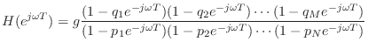
Now consider what happens when we take the factored form of the
general transfer function, Eq.![]() (8.2), and set
(8.2), and set ![]() to
to
![]() to get the frequency response in factored form:
to get the frequency response in factored form:
In the complex plane, the number
![]() is plotted at the
coordinates
is plotted at the
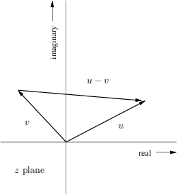
coordinates ![]() [84]. The difference of two vectors
[84]. The difference of two vectors
![]() and
and
![]() is
is
![]() , as shown in Fig.8.1. Translating the origin of the
vector
, as shown in Fig.8.1. Translating the origin of the
vector ![]() to the tip of
to the tip of ![]() shows that
shows that ![]() is an arrow drawn
from the tip of
is an arrow drawn
from the tip of ![]() to the tip of
to the tip of ![]() . The length of a vector is
unaffected by translation away from the origin. However, the angle of
a translated vector must be measured relative to a translated copy of
the real axis. Thus the term
. The length of a vector is
unaffected by translation away from the origin. However, the angle of
a translated vector must be measured relative to a translated copy of
the real axis. Thus the term
![]() may be drawn as an
arrow from the
may be drawn as an
arrow from the ![]() th zero to the point
th zero to the point
![]() on the unit
circle, and
on the unit
circle, and
![]() is an arrow from the
is an arrow from the ![]() th
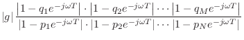
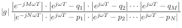
pole. Therefore, each term in Eq.
th
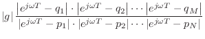
pole. Therefore, each term in Eq.![]() (8.3) is the length
of a vector drawn from a pole or zero to a single point on the unit
circle, as shown in Fig.8.2 for two poles and two zeros.
In summary:
(8.3) is the length
of a vector drawn from a pole or zero to a single point on the unit
circle, as shown in Fig.8.2 for two poles and two zeros.
In summary:
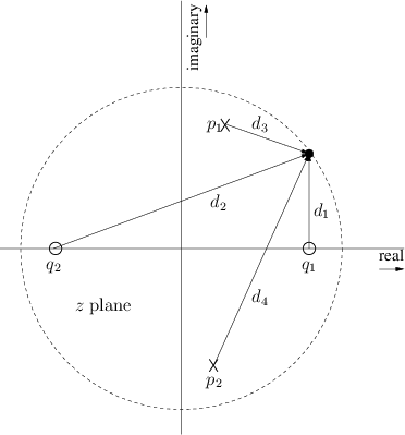 |
For example, the dc gain is obtained by multiplying the lengths of the
lines drawn from all poles and zeros to the point ![]() . The filter
gain at half the sampling rate is the product of the lengths of these
lines when drawn to the point
. The filter
gain at half the sampling rate is the product of the lengths of these
lines when drawn to the point ![]() . For an arbitrary frequency
. For an arbitrary frequency
![]() Hz, we draw arrows from the poles and zeros to the point
Hz, we draw arrows from the poles and zeros to the point
![]() . Thus, at the frequency where the arrows in
Fig.8.2 join, (which is slightly less than one-eighth the
sampling rate) the gain of this two-pole two-zero filter is
. Thus, at the frequency where the arrows in
Fig.8.2 join, (which is slightly less than one-eighth the
sampling rate) the gain of this two-pole two-zero filter is
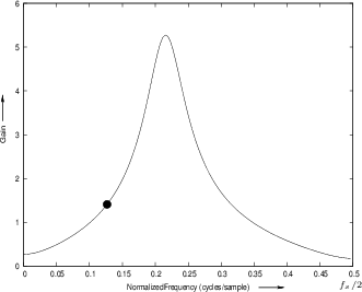
![]() . Figure 8.3 gives the complete amplitude
response for the poles and zeros shown in Fig.8.2. Before
looking at that, it is a good exercise to try sketching it by
inspection of the pole-zero diagram. It is usually easy to sketch a
qualitatively accurate amplitude-response directly from the poles and
zeros (to within a scale factor).
. Figure 8.3 gives the complete amplitude
response for the poles and zeros shown in Fig.8.2. Before
looking at that, it is a good exercise to try sketching it by
inspection of the pole-zero diagram. It is usually easy to sketch a
qualitatively accurate amplitude-response directly from the poles and
zeros (to within a scale factor).
 |
Next Section:
Graphical Phase Response Calculation
Previous Section:
Filter Order = Transfer Function Order


