


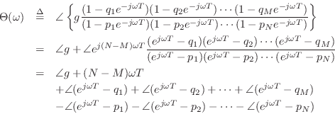
Graphical Phase Response Calculation
The phase response is almost as easy to evaluate graphically as is the amplitude response:
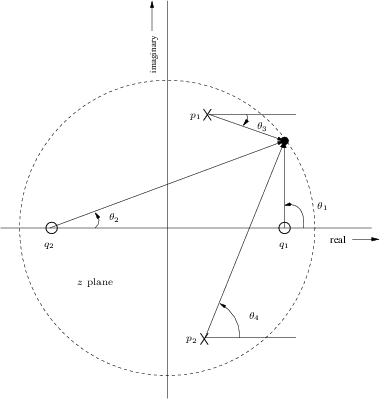
If ![]() is real, then
is real, then ![]() is either 0 or
is either 0 or ![]() . Terms of the
form
. Terms of the
form
![]() can be interpreted as a vector drawn from the point
can be interpreted as a vector drawn from the point ![]() to the point
to the point
![]() in the complex plane. The angle of
in the complex plane. The angle of
![]() is
the angle of the constructed vector (where a vector pointing
horizontally to the right has an angle of 0). Therefore, the phase
response at frequency
is
the angle of the constructed vector (where a vector pointing
horizontally to the right has an angle of 0). Therefore, the phase
response at frequency ![]() Hz is again obtained by drawing lines from
all the poles and zeros to the point
Hz is again obtained by drawing lines from
all the poles and zeros to the point
![]() , as shown in
Fig.8.4. The angles of the lines from the zeros are added, and
the angles of the lines from the poles are subtracted. Thus, at the
frequency
, as shown in
Fig.8.4. The angles of the lines from the zeros are added, and
the angles of the lines from the poles are subtracted. Thus, at the
frequency ![]() the phase response of the two-pole two-zero filter
in the figure is
the phase response of the two-pole two-zero filter
in the figure is
![]() .
.
Note that an additional phase of
![]() radians appears when
the number of poles is not equal to the number of zeros. This factor
comes from writing the transfer function as
radians appears when
the number of poles is not equal to the number of zeros. This factor
comes from writing the transfer function as
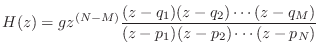
 |
Next Section:
Stability Revisited
Previous Section:
Graphical Computation of Amplitude Response from Poles and Zeros


