Markov Parameters

The impulse response of a state-space model is easily found by direct calculation using Eq.(G.1):

Note that we have assumed (zero initial state or zero initial conditions). The notation denotes a matrix having along the diagonal and zeros elsewhere.^G.2

The impulse response of the state-space model can be summarized as

The impulse response terms for are known as the Markov parameters of the state-space model.

Note that each sample of the impulse response is a matrix.^G.3 Therefore, it is not a possible output signal, except when . A better name might be ``impulse-matrix response''. In §G.4 below, we'll see that is the inverse z transform of the matrix transfer-function of the system.

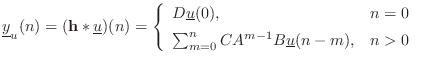
Given an arbitrary input signal (and zero intial conditions ), the output signal is given by the convolution of the input signal with the impulse response:

---

Order a Hardcopy of Introduction to Digital Filters

Previous: State Space Filters
Next: Response from Initial Conditions

---

written by Julius Orion Smith III
Julius Smith's background is in electrical engineering (BS Rice 1975, PhD Stanford 1983). He is presently Professor of Music and Associate Professor (by courtesy) of Electrical Engineering at Stanford's Center for Computer Research in Music and Acoustics (CCRMA), teaching courses and pursuing research related to signal processing applied to music and audio systems. See http://ccrma.stanford.edu/~jos/ for details.