


Numerical Computation of Group Delay
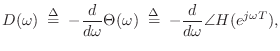
The definition of group delay,
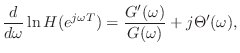
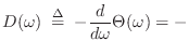
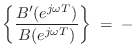
A more useful form of the group delay arises from the
logarithmic derivative of the frequency response. Expressing
the frequency response
![]() in polar form as
in polar form as
Since differentiation is linear, the logarithmic derivative becomes
 im
im im
im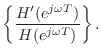
In this case, the derivative is simply
![\begin{eqnarray*}
B^\prime(e^{j\omega T}) &\isdef & \frac{d}{d\omega}\left[b_0
...
...b_M e^{-jM\omega T}\right]\\
&\isdef & -jT\,B_r(e^{j\omega T}),
\end{eqnarray*}](http://www.dsprelated.com/josimages_new/filters/img947.png)
where ![]() denotes ``
denotes ``![]() ramped'', i.e., the
ramped'', i.e., the ![]() th coefficient of
the polynomial
th coefficient of
the polynomial ![]() is
is ![]() , for
, for
![]() . In
matlab, we may compute Br from B via the
following statement:
. In
matlab, we may compute Br from B via the
following statement:
Br = B .* [0:M]; % Compute ramped B polynomialThe group delay of an FIR filter
 im
im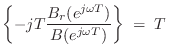 re
re
D = real(fft(Br) ./ fft(B))where the fft, of course, approximates the Discrete Time Fourier Transform (DTFT). Such sampling of the frequency axis by this approximation is information-preserving whenever the number of samples (FFT length) exceeds the polynomial order
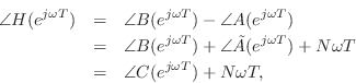
Finally, when there are both poles and zeros, we have
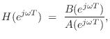
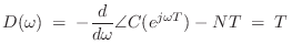
Straightforward differentiation yields
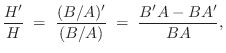
and this can be implemented analogous to the FIR case discussed above. However, a faster algorithm (usually) results from converting the IIR case to the FIR case:
where
C = conv(B,fliplr(conj(A)));It is straightforward to show (Problem 11) that
and the group delay computation thus reduces to the FIR case:
 re
re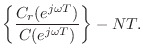
Next Section:
Computing Reflection Coefficients to Check Filter Stability
Previous Section:
Vocoder Analysis


