


Polar Form of the Frequency Response
When the complex-valued frequency response is expressed in polar form, the amplitude response and phase response explicitly appear:
Writing the basic frequency response description
![\begin{eqnarray*}
Y(e^{j\omega T}) &=& \left\vert Y(e^{j\omega T})\right\vert e^...
...ight\vert\right]
e^{j[\angle X(e^{j\omega T})+ \Theta(\omega)]}
\end{eqnarray*}](http://www.dsprelated.com/josimages_new/filters/img846.png)
which implies
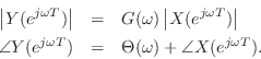
This states explicitly that the output magnitude spectrum equals the
input magnitude spectrum times the filter amplitude response,
and the output phase equals the input phase plus the filter
phase at each frequency ![]() .
.
Equation (7.3) gives the frequency response in polar form. For completeness, recall the transformations between polar and rectangular forms (i.e., for converting real and imaginary parts to magnitude and angle, and vice versa):
![\begin{eqnarray*}
G(\omega) &\isdef & \left\vert H(e^{j\omega T})\right\vert \eq...
...ga T})\right\}}{\mbox{re}\left\{H(e^{j\omega T})\right\}}\right]
\end{eqnarray*}](http://www.dsprelated.com/josimages_new/filters/img848.png)
Going the other way from polar to rectangular (using Euler's formula),
![\begin{eqnarray*}
\mbox{re}\left\{H(e^{j\omega T})\right\} &=& G(\omega) \cos[\T...
...ft\{H(e^{j\omega T})\right\} &=& G(\omega) \sin[\Theta(\omega)].
\end{eqnarray*}](http://www.dsprelated.com/josimages_new/filters/img849.png)
Application of these formulas to some basic example filters are carried out in Appendix B. Some useful trig identities are summarized in Appendix A. A matlab listing for computing the frequency response of any IIR filter is given in §7.5.1 below.
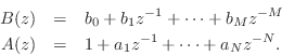
Separating the Transfer Function Numerator and Denominator
From Eq.![]() (6.5) we have that the transfer function of a
recursive filter is a ratio of polynomials in
(6.5) we have that the transfer function of a
recursive filter is a ratio of polynomials in ![]() :
:

where
By elementary properties of complex numbers, we have
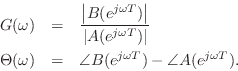
These relations can be used to simplify calculations by hand, allowing the numerator and denominator of the transfer function to be handled separately.
Next Section:
Frequency Response as a Ratio of DTFTs
Previous Section:
Phase Response


