State Space Simulation in Matlab

Since matlab has first-class support for matrices and vectors, it is quite simple to implement a state-space model in Matlab using no support functions whatsoever, e.g.,

% Define the state-space system parameters:
A = [0 1; -1 0]; % State transition matrix
B = [0; 1];  C = [0 1];  D = 0; % Input, output, feed-around

% Set up the input signal, initial conditions, etc.
x0 = [0;0];             % Initial state (N=2)
Ns = 10; 	        % Number of sample times to simulate
u = [1, zeros(1,Ns-1)]; % Input signal (an impulse at time 0)
y = zeros(Ns,1);        % Preallocate output signal for n=0:Ns-1

% Perform the system simulation:
x = x0;                % Set initial state
for n=1:Ns-1           % Iterate through time
  y(n) = C*x + D*u(n); % Output for time n-1
  x = A*x + B*u(n);    % State transitions to time n
end
y' % print the output y (transposed)
% ans =
%  0   1   0  -1   0   1   0  -1   0   0

The restriction to indexes beginning at 1 is unwieldy here, because we want to include time in the input and output. It can be readily checked that the above examples has the transfer function

so that the following matlab checks the above output using the built-in filter function:

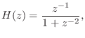
NUM = [0 1];
DEN = [1 0 1];
y = filter(NUM,DEN,u)
% y =
%   0   1   0  -1   0   1   0  -1   0   1

To eliminate the unit-sample delay, i.e., to simulate in state-space form, it is necessary to use the (feed-around) coefficient:

[A,B,C,D] = tf2ss([1 0 0], [1 0 1])
% A =
%    0   1
%   -1  -0
%
% B =
%   0
%   1
%
% C =
%   -1   0
%
% D = 1

x = x0;                % Reset to initial state
for n=1:Ns-1
  y(n) = C*x + D*u(n);
  x = A*x + B*u(n);
end
y'
% ans =
%  1   0  -1   0   1   0  -1   0   1   0

Note the use of trailing zeros in the first argument of tf2ss (the transfer-function numerator-polynomial coefficients) to make it the same length as the second argument (denominator coefficients). This is necessary in tf2ss because the same function is used for both the continous- and discrete-time cases. Without the trailing zeros, the numerator will be extended by zeros on the left, i.e., ``right-justified'' relative to the denominator.

---

Previous: Matlab Direct-Form to State-Space Conversion
Next: Other Relevant Matlab Functions

Order a Hardcopy of Introduction to Digital Filters

---

About the Author: Julius Orion Smith III
Julius Smith's background is in electrical engineering (BS Rice 1975, PhD Stanford 1983). He is presently Professor of Music and Associate Professor (by courtesy) of Electrical Engineering at Stanford's Center for Computer Research in Music and Acoustics (CCRMA), teaching courses and pursuing research related to signal processing applied to music and audio systems. See http://ccrma.stanford.edu/~jos/ for details.