


Two-Zero
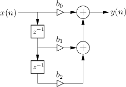
The signal flow graph for the general two-zero filter is given in Fig.B.7, and the derivation of frequency response is as follows:
![\fbox{
\begin{tabular}{rl}
Difference equation: & $y(n) = b_0 x(n) + b_1 x(n-1) ...
...+ b_1 \cos(\omega T) + b_2 \cos(2\omega T)}\right]$
\end{tabular}\vspace{10pt}
}](http://www.dsprelated.com/josimages_new/filters/img1389.png)
As discussed in §5.1,
the parameters ![]() and
and ![]() are called the numerator
coefficients, and they determine the two zeros. Using the
quadratic formula for finding the roots of a second-order polynomial,
we find that the zeros are located at
are called the numerator
coefficients, and they determine the two zeros. Using the
quadratic formula for finding the roots of a second-order polynomial,
we find that the zeros are located at

Forming a general two-zero transfer function in factored form gives
![\begin{eqnarray*}
H(z) &=& b_0 (1 - Re^{j\theta_c} z^{-1}) (1 - Re^{-j\theta_c} z^{-1})\\
&=& b_0 [1 - 2R\cos(\theta_c) z^{-1}+ R^2 z^{-2}]
\end{eqnarray*}](http://www.dsprelated.com/josimages_new/filters/img1397.png)
from which we identify
![]() and
and
![]() , so that
, so that
The approximate relation between bandwidth and ![]() given in
Eq.
given in
Eq.![]() (B.5) for the two-pole resonator now applies to the notch
width in the two-zero filter.
(B.5) for the two-pole resonator now applies to the notch
width in the two-zero filter.
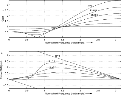
Figure B.8 gives some two-zero frequency responses obtained by
setting ![]() to 1 and varying
to 1 and varying ![]() . The value of
. The value of ![]() , is again
, is again
![]() . Note that the response is exactly analogous to the two-pole
resonator with notches replacing the resonant peaks. Since the plots
are on a linear magnitude scale, the two-zero amplitude response
appears as the reciprocal of a two-pole response. On a dB scale, the
two-zero response is an upside-down two-pole response.
. Note that the response is exactly analogous to the two-pole
resonator with notches replacing the resonant peaks. Since the plots
are on a linear magnitude scale, the two-zero amplitude response
appears as the reciprocal of a two-pole response. On a dB scale, the
two-zero response is an upside-down two-pole response.
 |
Next Section:
Complex Resonator
Previous Section:
Two-Pole


