Z Transform of Difference Equations

Since z transforming the convolution representation for digital filters was so fruitful, let's apply it now to the general difference equation, Eq. $\,$ (5.1). To do this requires two properties of the z transform, linearity (easy to show) and the shift theorem (derived in §6.3 above). Using these two properties, we can write down the z transform of any difference equation by inspection, as we now show. In §6.8.2, we'll show how to invert by inspection as well.

Repeating the general difference equation for LTI filters, we have (from Eq. $\,$ (5.1)) $\begin{eqnarrayda} y(n) &=& b_0 x(n) &+& b_1 x(n - 1) + \cdots + b_M x(n - M)\\ & & &-& a_1 y(n - 1) - \cdots - a_N y(n - N).\\ \end{eqnarrayda}$

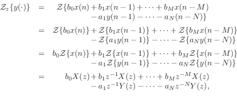Let's take the z transform of both sides, denoting the transform by ${\cal Z}\{\}$ . Because ${\cal Z}\{\}$ is a linear operator, it may be distributed through the terms on the right-hand side as follows:^7.3 $\begin{eqnarrayda} {\cal Z}_z\{y(\cdot)\} &=& {\cal Z}\{ b_0 x(n) &+& b_1 x(n ... ...-M} X(z)\\ & & &-& a_1 z^{-1}Y(z) - \cdots - a_N z^{-N} Y(z), \end{eqnarrayda}$ where we used the superposition and scaling properties of linearity given on page , followed by use of the shift theorem, in that order. The terms in may be grouped together on the left-hand side to get

$\begin{eqnarray*} \lefteqn{Y(z) + a_1 z^{-1}Y(z) + \cdots + a_N z^{-N} Y(z) = }\... ... \\ & & b_0 X(z) + b_1 z^{-1}X(z) + \cdots + b_M z^{-M} X(z). \end{eqnarray*}$

Factoring out the common terms and gives

$\displaystyle Y(z)\left[1 + a_1 z^{-1}+ \cdots + a_N z^{-N}\right] = X(z)\left[b_0 + b_1 z^{-1}+ \cdots + b_M z^{-M}\right].$

Defining the polynomials

$\begin{eqnarray*} A(z) &\isdef & 1 + a_1\,z^{-1} + \,\cdots\, + a_N\,z^{-N}\\ B(z) &\isdef & b_0 + b_1\,z^{-1}+\,\cdots\,+b_M\,z^{-M}, \end{eqnarray*}$

the z transform of the difference equation yields

$\displaystyle A(z)\,Y(z) = B(z)\,X(z).$

Finally, solving for

, which is by definition the transfer function

, gives

$\displaystyle H(z) \isdefs \frac{Y(z)}{X(z)} \eqsp \frac{b_0 + b_1 z^{-1}+ \cdo... ...^{-M}}{1 + a_1 z^{-1}+ \cdots + a_N z^{-N}} \isdefs \frac{B(z)}{A(z)}. \protect$

(7.5)

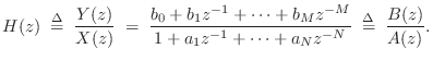
Thus, taking the z transform of the general difference equation led to a new formula for the transfer function in terms of the difference equation coefficients. (Now the minus signs for the feedback coefficients in the difference equation Eq. $\,$ (5.1) are explained.)

Order a Hardcopy of Introduction to Digital Filters

Previous: Z Transform of Convolution
Next: Factored Form

written by Julius Orion Smith III
Julius Smith's background is in electrical engineering (BS Rice 1975, PhD Stanford 1983). He is presently Professor of Music and Associate Professor (by courtesy) of Electrical Engineering at Stanford's Center for Computer Research in Music and Acoustics (CCRMA), teaching courses and pursuing research related to signal processing applied to music and audio systems. See http://ccrma.stanford.edu/~jos/ for details.

Sign in

Search Online Books

Free Online Books

Sponsor

Chapters

See Also

Introduction to Digital Filters
Transfer Function Analysis
Z Transform of Difference Equations