


Coherence Function
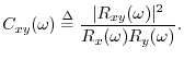
A function related to cross-correlation is the coherence function, defined in terms of power spectral densities and the cross-spectral density by

The coherence
![]() is a real function between zero and one
which gives a measure of correlation between
is a real function between zero and one
which gives a measure of correlation between ![]() and
and ![]() at
each frequency
at
each frequency ![]() . For example, imagine that
. For example, imagine that ![]() is produced
from
is produced
from ![]() via an LTI filtering operation:
via an LTI filtering operation:
so that the coherence function becomes

A common use for the coherence function is in the validation of
input/output data collected in an acoustics experiment for purposes of
system identification. For example, ![]() might be a known
signal which is input to an unknown system, such as a reverberant
room, say, and
might be a known
signal which is input to an unknown system, such as a reverberant
room, say, and ![]() is the recorded response of the room. Ideally,
the coherence should be
is the recorded response of the room. Ideally,
the coherence should be ![]() at all frequencies. However, if the
microphone is situated at a null in the room response for some
frequency, it may record mostly noise at that frequency. This is
indicated in the measured coherence by a significant dip below 1. An
example is shown in Book III [69] for the case of a measured
guitar-bridge admittance.
A more elementary example is given in the next section.
at all frequencies. However, if the
microphone is situated at a null in the room response for some
frequency, it may record mostly noise at that frequency. This is
indicated in the measured coherence by a significant dip below 1. An
example is shown in Book III [69] for the case of a measured
guitar-bridge admittance.
A more elementary example is given in the next section.
Coherence Function in Matlab
In Matlab and Octave, cohere(x,y,M) computes the coherence
function ![]() using successive DFTs of length
using successive DFTs of length ![]() with a Hanning
window and 50% overlap. (The window and overlap can be controlled
via additional optional arguments.) The matlab listing in
Fig.8.14 illustrates cohere on a simple example.
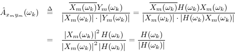
Figure 8.15 shows a plot of cxyM for this example.
We see a coherence peak at frequency
with a Hanning
window and 50% overlap. (The window and overlap can be controlled
via additional optional arguments.) The matlab listing in
Fig.8.14 illustrates cohere on a simple example.
Figure 8.15 shows a plot of cxyM for this example.
We see a coherence peak at frequency ![]() cycles/sample, as
expected, but there are also two rather large coherence samples on
either side of the main peak. These are expected as well, since the
true cross-spectrum for this case is a critically sampled Hanning
window transform. (A window transform is critically sampled whenever
the window length equals the DFT length.)
cycles/sample, as
expected, but there are also two rather large coherence samples on
either side of the main peak. These are expected as well, since the
true cross-spectrum for this case is a critically sampled Hanning
window transform. (A window transform is critically sampled whenever
the window length equals the DFT length.)
% Illustrate estimation of coherence function 'cohere' % in the Matlab Signal Processing Toolbox % or Octave with Octave Forge: N = 1024; % number of samples x=randn(1,N); % Gaussian noise y=randn(1,N); % Uncorrelated noise f0 = 1/4; % Frequency of high coherence nT = [0:N-1]; % Time axis w0 = 2*pi*f0; x = x + cos(w0*nT); % Let something be correlated p = 2*pi*rand(1,1); % Phase is irrelevant y = y + cos(w0*nT+p); M = round(sqrt(N)); % Typical window length [cxyM,w] = cohere(x,y,M); % Do the work figure(1); clf; stem(w/2,cxyM,'*'); % w goes from 0 to 1 (odd convention) legend(''); % needed in Octave grid on; ylabel('Coherence'); xlabel('Normalized Frequency (cycles/sample)'); axis([0 1/2 0 1]); replot; % Needed in Octave saveplot('../eps/coherex.eps'); % compatibility utility |
![\includegraphics[width=\twidth]{eps/coherex}](http://www.dsprelated.com/josimages_new/mdft/img1617.png)
Note that more than one frame must be averaged to obtain a coherence
less than one. For example, changing the cohere call in the
above example to
``cxyN = cohere(x,y,N);''
produces all ones in cxyN, because no averaging is
performed.
Next Section:
Recommended Further Reading
Previous Section:
Power Spectral Density Estimation


