


Convolution Example 2: ADSR Envelope
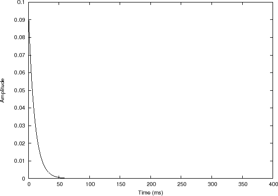
Filter impulse response 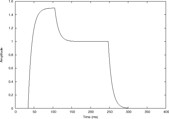
Filter output signal |
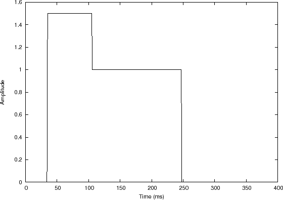
In this example, the input signal is a sequence of two rectangular pulses, creating a piecewise constant function, depicted in Fig.7.4(a). The filter impulse response, shown in Fig.7.4(b), is a truncated exponential.7.6
In this example, ![]() is again a causal smoothing-filter impulse
response, and we could call it a ``moving weighted average'', in which
the weighting is exponential into the past. The discontinuous steps
in the input become exponential ``asymptotes'' in the output which are
approached exponentially. The overall appearance of the output signal
resembles what is called an attack, decay, release, and sustain
envelope, or ADSR envelope for short. In a practical ADSR
envelope, the time-constants for attack, decay, and release may be set
independently. In this example, there is only one time constant, that
of
is again a causal smoothing-filter impulse
response, and we could call it a ``moving weighted average'', in which
the weighting is exponential into the past. The discontinuous steps
in the input become exponential ``asymptotes'' in the output which are
approached exponentially. The overall appearance of the output signal
resembles what is called an attack, decay, release, and sustain
envelope, or ADSR envelope for short. In a practical ADSR
envelope, the time-constants for attack, decay, and release may be set
independently. In this example, there is only one time constant, that
of ![]() . The two constant levels in the input signal may be called the
attack level and the sustain level, respectively. Thus,
the envelope approaches the attack level at the attack rate (where the
``rate'' may be defined as the reciprocal of the time constant), it
next approaches the sustain level at the ``decay rate'', and finally,
it approaches zero at the ``release rate''. These envelope parameters
are commonly used in analog synthesizers and their digital
descendants, so-called virtual analog synthesizers. Such an
ADSR envelope is typically used to multiply the output of a waveform
oscillator such as a sawtooth or pulse-train oscillator. For more on
virtual analog synthesis, see, for example,
[78,77].
. The two constant levels in the input signal may be called the
attack level and the sustain level, respectively. Thus,
the envelope approaches the attack level at the attack rate (where the
``rate'' may be defined as the reciprocal of the time constant), it
next approaches the sustain level at the ``decay rate'', and finally,
it approaches zero at the ``release rate''. These envelope parameters
are commonly used in analog synthesizers and their digital
descendants, so-called virtual analog synthesizers. Such an
ADSR envelope is typically used to multiply the output of a waveform
oscillator such as a sawtooth or pulse-train oscillator. For more on
virtual analog synthesis, see, for example,
[78,77].
Next Section:
Convolution Example 3: Matched Filtering
Previous Section:
Convolution Example 1: Smoothing a Rectangular Pulse


