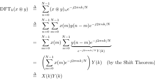
Convolution Theorem

Theorem: For any ,

Proof:

This is perhaps the most important single Fourier theorem of all. It is the basis of a large number of FFT applications. Since an FFT provides a fast Fourier transform, it also provides fast convolution, thanks to the convolution theorem. It turns out that using an FFT to perform convolution is really more efficient in practice only for reasonably long convolutions, such as . For much longer convolutions, the savings become enormous compared with ``direct'' convolution. This happens because direct convolution requires on the order of operations (multiplications and additions), while FFT-based convolution requires on the order of operations, where denotes the logarithm-base-2 of (see §A.1.2 for an explanation).

The simple matlab example in Fig.7.13 illustrates how much faster convolution can be performed using an FFT.^7.16 We see that for a length convolution, the fft function is approximately 300 times faster in Octave, and 30 times faster in Matlab. (The conv routine is much faster in Matlab, even though it is a built-in function in both cases.)

N = 1024;        % FFT much faster at this length
t = 0:N-1;       % [0,1,2,...,N-1]
h = exp(-t);     % filter impulse reponse
H = fft(h);      % filter frequency response
x = ones(1,N);   % input = dc (any signal will do)
Nrep = 100;      % number of trials to average
t0 = clock;      % latch the current time
for i=1:Nrep, y = conv(x,h); end      % Direct convolution
t1 = etime(clock,t0)*1000; % elapsed time in msec
t0 = clock; 
for i=1:Nrep, y = ifft(fft(x) .* H); end % FFT convolution
t2 = etime(clock,t0)*1000;
disp(sprintf([...
    'Average direct-convolution time = %0.2f msec\n',...
    'Average FFT-convolution time = %0.2f msec\n',...
    'Ratio = %0.2f (Direct/FFT)'],...
    t1/Nrep,t2/Nrep,t1/t2));

% =================== EXAMPLE RESULTS ===================

Octave:
Average direct-convolution time = 69.49 msec
Average FFT-convolution time = 0.23 msec
Ratio = 296.40 (Direct/FFT)

Matlab:
Average direct-convolution time = 15.73 msec
Average FFT-convolution time = 0.50 msec
Ratio = 31.46 (Direct/FFT)

A similar program produced the results for different FFT lengths shown in Table 7.1.^7.17 In this software environment, the fft function is faster starting with length , and it is never significantly slower at short lengths, where ``calling overhead'' dominates.

Table 7.1: Direct versus FFT convolution times in milliseconds (convolution length = ) using Matlab 5.2 on an 800 MHz Athlon Windows PC.

M Direct FFT Ratio 1 0.07 0.08 0.91 2 0.08 0.08 0.92 3 0.08 0.08 0.94 4 0.09 0.10 0.97 5 0.12 0.12 0.96 6 0.18 0.12 1.44 7 0.39 0.15 2.67 8 1.10 0.21 5.10 9 3.83 0.31 12.26 10 15.80 0.47 33.72 11 50.39 1.09 46.07 12 177.75 2.53 70.22 13 709.75 5.62 126.18 14 4510.25 17.50 257.73 15 19050.00 72.50 262.76 16 316375.00 440.50 718.22

A table similar to Table 7.1 in Strum and Kirk [76, p. 521], based on the number of real multiplies, finds that the fft is faster starting at length , and that direct convolution is significantly faster for very short convolutions (e.g., 16 operations for a direct length-4 convolution, versus 176 for the fft function).

See Appendix A for further discussion of FFT algorithms and their applications.

Order a Hardcopy of Mathematics of the DFT