


Example AM Spectra
Equation (4.4) can be used to write down the spectral representation of
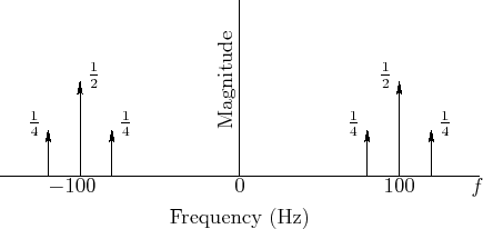
![]() by inspection, as shown in Fig.4.12. In the example
of Fig.4.12, we have
by inspection, as shown in Fig.4.12. In the example
of Fig.4.12, we have ![]() Hz and
Hz and ![]() Hz,
where, as always,
Hz,
where, as always,
![]() . For comparison, the spectral
magnitude of an unmodulated
. For comparison, the spectral
magnitude of an unmodulated ![]() Hz sinusoid is shown in
Fig.4.6. Note in Fig.4.12 how each of the two
sinusoidal components at
Hz sinusoid is shown in
Fig.4.6. Note in Fig.4.12 how each of the two
sinusoidal components at ![]() Hz have been ``split'' into two
``side bands'', one
Hz have been ``split'' into two
``side bands'', one ![]() Hz higher and the other
Hz higher and the other ![]() Hz lower, that
is,
Hz lower, that
is,
![]() . Note also how the
amplitude of the split component is divided equally among its
two side bands.
. Note also how the
amplitude of the split component is divided equally among its
two side bands.

Recall that ![]() was defined as the second term of
Eq.
was defined as the second term of
Eq.![]() (4.1). The first term is simply the original unmodulated
signal. Therefore, we have effectively been considering AM with a
``very large'' modulation index. In the more general case of
Eq.
(4.1). The first term is simply the original unmodulated
signal. Therefore, we have effectively been considering AM with a
``very large'' modulation index. In the more general case of
Eq.![]() (4.1) with
(4.1) with ![]() given by Eq.
given by Eq.![]() (4.2), the magnitude of
the spectral representation appears as shown in Fig.4.13.
(4.2), the magnitude of
the spectral representation appears as shown in Fig.4.13.
Next Section:
Bessel Functions


