Power Spectral Density Estimation

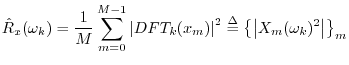
Welch's method [82] (or the periodogram method [18]) for estimating power spectral densities (PSD) is carried out by dividing the time signal into successive blocks, and averaging squared-magnitude DFTs of the signal blocks. Let , $n=0,1,\dots,N-1$ , denote the th block of the signal $x\in{\bf C}^{MN}$ , with denoting the number of blocks. Then the Welch PSD estimate is given by

$\displaystyle {\hat R}_x(\omega_k) = \frac{1}{M}\sum_{m=0}^{M-1}\left\vert DFT_... ...t\vert^2 \isdef \left\{\left\vert X_m(\omega_k)^2\right\vert\right\}_m \protect$

(8.3)

where `` $\{\cdot\}_m$ '' denotes time averaging across blocks (or ``frames'') of data indexed by

. The function pwelch implements Welch's method in Octave (Octave-Forge collection) and Matlab (Signal Processing Toolbox).

Recall that $\left\vert X_m\right\vert^2\;\leftrightarrow\;x\star x$ which is circular (cyclic) autocorrelation. To obtain an acyclic autocorrelation instead, we may use zero padding in the time domain, as described in §8.4.2. That is, we can replace above by $\hbox{\sc CausalZeroPad}_{2N-1}(x_m) = [x_m,0,\ldots,0]$ .^8.9Although this fixes the ``wrap-around problem'', the estimator is still biased because its expected value is the true autocorrelation weighted by $N-\vert l\vert$ . This bias is equivalent to multiplying the correlation in the ``lag domain'' by a triangular window (also called a ``Bartlett window''). The bias can be removed by simply dividing it out, as in Eq. $\,$ (8.2), but it is common to retain the Bartlett weighting since it merely corresponds to smoothing the power spectrum (or cross-spectrum) with a sinc kernel;^8.10it also down-weights the less reliable large-lag estimates, weighting each lag by the number of lagged products that were summed.

Since $\vert X_m(\omega_k)\vert^2=N\cdot\hbox{\sc DFT}_k({\hat r}_{x_m})$ , and since the DFT is a linear operator (§7.4.1), averaging magnitude-squared DFTs $\vert X_m(\omega_k)\vert^2$ is equivalent, in principle, to estimating block autocorrelations ${\hat r}_{x_m}$ , averaging them, and taking a DFT of the average. However, this would normally be slower.

We return to power spectral density estimation in Book IV [67] of the music signal processing series.

Order a Hardcopy of Mathematics of the DFT

Previous: FIR System Identification
Next: Coherence Function

written by Julius Orion Smith III
Julius Smith's background is in electrical engineering (BS Rice 1975, PhD Stanford 1983). He is presently Professor of Music and Associate Professor (by courtesy) of Electrical Engineering at Stanford's Center for Computer Research in Music and Acoustics (CCRMA), teaching courses and pursuing research related to signal processing applied to music and audio systems. See http://ccrma.stanford.edu/~jos/ for details.

Sign in

Search Online Books

Free Online Books

Ads

Chapters

See Also

Mathematics of the DFT
Example Applications of the DFT
Power Spectral Density Estimation