Round-Off Error Variance

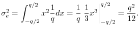
This appendix shows how to derive that the noise power of amplitude quantization error is , where is the quantization step size. This is an example of a topic in statistical signal processing, which is beyond the scope of this book. (Some good textbooks in this area include [27,51,34,33,65,32].) However, since the main result is so useful in practice, it is derived below anyway, with needed definitions given along the way. The interested reader is encouraged to explore one or more of the above-cited references in statistical signal processing.^G.10

Each round-off error in quantization noise is modeled as a uniform random variable between and . It therefore has the following probability density function (pdf) [51]:^G.11

$\displaystyle p_e(x) = \left\{\begin{array}{ll} \frac{1}{q}, & \left\vert x\ri... ...2} \\ [5pt] 0, & \left\vert x\right\vert>\frac{q}{2} \\ \end{array} \right.$

Thus, the probability that a given roundoff error

lies in the interval

is given by

$\displaystyle \int_{x_1}^{x_2} p_e(x) dx = \frac{x_2-x_1}{q}$

assuming of course that

and

lie in the allowed range

. We might loosely refer to

as a probability distribution, but technically it is a probability density function, and to obtain probabilities, we have to integrate over one or more intervals, as above. We use probability distributions for variables which take on discrete values (such as dice), and we use probability densities for variables which take on continuous values (such as round-off errors).

The mean of a random variable is defined as

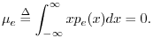
$\displaystyle \mu_e \isdef \int_{-\infty}^{\infty} x p_e(x) dx = 0.$

In our case, the mean is zero because we are assuming the use of rounding (as opposed to truncation, etc.).

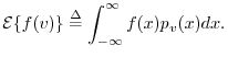
The mean of a signal is the same thing as the expected value of , which we write as ${\cal E}\{e(n)\}$ . In general, the expected value of any function of a random variable is given by

$\displaystyle {\cal E}\{f(v)\} \isdef \int_{-\infty}^{\infty} f(x) p_v(x) dx.$

Since the quantization-noise signal is modeled as a series of independent, identically distributed (iid) random variables, we can estimate the mean by averaging the signal over time. Such an estimate is called a sample mean.

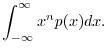
Probability distributions are often characterized by their moments. The th moment of the pdf is defined as

$\displaystyle \int_{-\infty}^{\infty} x^n p(x) dx.$

Thus, the mean $\mu_x = {\cal E}\{e(n)\}$ is the first moment of the pdf. The second moment is simply the expected value of the random variable squared, i.e., ${\cal E}\{e^2(n)\}$ .

The variance of a random variable is defined as the second central moment of the pdf:

$\displaystyle \sigma_e^2 \isdef {\cal E}\{[e(n)-\mu_e]^2\} = \int_{-\infty}^{\infty} (x-\mu_e)^2 p_e(x) dx$

``Central'' just means that the moment is evaluated after subtracting out the mean, that is, looking at $e(n)-\mu_e$ instead of

. In the case of round-off errors, the mean is zero, so subtracting out the mean has no effect. Plugging in the constant pdf for our random variable

which we assume is uniformly distributed on

, we obtain the variance

$\displaystyle \sigma_e^2 = \int_{-q/2}^{q/2} x^2 \frac{1}{q} dx = \frac{1}{q}\left.\frac{1}{3}x^3\right\vert _{-q/2}^{q/2} = \frac{q^2}{12}.$

Note that the variance of

can be estimated by averaging

over time, that is, by computing the mean square. Such an estimate is called the sample variance. For sampled physical processes, the sample variance is proportional to the average power in the signal. Finally, the square root of the sample variance (the rms level) is sometimes called the standard deviation of the signal, but this term is only precise when the random variable has a Gaussian pdf.

Previous: Mu-Law Coding
Next: Matrices

Order a Hardcopy of Mathematics of the DFT

About the Author: Julius Orion Smith III
Julius Smith's background is in electrical engineering (BS Rice 1975, PhD Stanford 1983). He is presently Professor of Music and Associate Professor (by courtesy) of Electrical Engineering at Stanford's Center for Computer Research in Music and Acoustics (CCRMA), teaching courses and pursuing research related to signal processing applied to music and audio systems. See http://ccrma.stanford.edu/~jos/ for details.

Sign in

Search Online Books

Free Online Books

Chapters

See Also

Mathematics of the DFT
Number Systems for Digital Audio
Round-Off Error Variance