


Acoustic Guitars
This section addresses some modeling considerations specific to acoustic guitars. Section 9.2.1 discusses special properties of acoustic guitar bridges, and §9.2.1 gives ways to simulate passive bridges, including a look at some laboratory measurements. For further reading in this area, see, e.g., [281,128].
Bridge Modeling
In §6.3 we analyzed the effect of rigid string terminations on traveling waves. We found that waves derived by time-derivatives of displacement (displacement, velocity, acceleration, and so on) reflect with a sign inversion, while waves defined in terms of the first spatial derivative of displacement (force, slope) reflect with no sign inversion. We now look at the more realistic case of yielding terminations for strings. This analysis can be considered a special case of the loaded string junction analyzed in §C.12.
Yielding string terminations (at the bridge) have a large effect on the sound produced by acoustic stringed instruments. Rigid terminations can be considered a reasonable model for the solid-body electric guitar in which maximum sustain is desired for played notes. Acoustic guitars, on the other hand, must transduce sound energy from the strings into the body of the instrument, and from there to the surrounding air. All audible sound energy comes from the string vibrational energy, thereby reducing the sustain (decay time) of each played note. Furthermore, because the bridge vibrates more easily in one direction than another, a kind of ``chorus effect'' is created from the detuning of the horizontal and vertical planes of string vibration (as discussed further in §6.12.1). A perfectly rigid bridge, in contrast, cannot transmit any sound into the body of the instrument, thereby requiring some other transducer, such as the magnetic pickups used in electric guitars, to extract sound for output.10.4
Passive String Terminations
When a traveling wave reflects from the bridge of a real stringed
instrument, the bridge moves, transmitting sound energy into the
instrument body. How far the bridge moves is determined by the
driving-point impedance of the bridge, denoted ![]() . The
driving point impedance is the ratio of Laplace transform of the force
on the bridge
. The
driving point impedance is the ratio of Laplace transform of the force
on the bridge ![]() to the velocity of motion that results
to the velocity of motion that results
![]() . That is,
. That is,
![]() .
.
For passive systems (i.e., for all unamplified acoustic musical
instruments), the driving-point impedance ![]() is positive
real (a property defined and discussed in §C.11.2). Being
positive real has strong implications on the nature of
is positive
real (a property defined and discussed in §C.11.2). Being
positive real has strong implications on the nature of ![]() . In
particular, the phase of
. In
particular, the phase of
![]() cannot exceed plus or minus
cannot exceed plus or minus
![]() degrees at any frequency, and in the lossless case, all poles and
zeros must interlace along the
degrees at any frequency, and in the lossless case, all poles and
zeros must interlace along the ![]() axis. Another
implication is that the reflectance of a passive bridge, as
seen by traveling waves on the string, is a so-called Schur
function (defined and discussed in §C.11); a Schur
reflectance is a stable filter having gain not exceeding 1 at any
frequency. In summary, a guitar bridge is passive if and only if its
driving-point impedance is positive real and (equivalently) its
reflectance is Schur. See §C.11 for a fuller discussion of
this point.
axis. Another
implication is that the reflectance of a passive bridge, as
seen by traveling waves on the string, is a so-called Schur
function (defined and discussed in §C.11); a Schur
reflectance is a stable filter having gain not exceeding 1 at any
frequency. In summary, a guitar bridge is passive if and only if its
driving-point impedance is positive real and (equivalently) its
reflectance is Schur. See §C.11 for a fuller discussion of
this point.
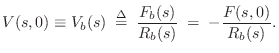
At ![]() , the force on the bridge is given by (§C.7.2)
, the force on the bridge is given by (§C.7.2)
A Terminating Resonator
Suppose a guitar bridge couples an ideal vibrating string to a single resonance, as depicted schematically in Fig.9.5. This is often an accurate model of an acoustic bridge impedance in a narrow frequency range, especially at low frequencies where the resonances are well separated. Then, as developed in Chapter 7, the driving-point impedance seen by the string at the bridge is
![\includegraphics[width=\twidth]{eps/f_yielding_term}](http://www.dsprelated.com/josimages_new/pasp/img1992.png) |
Bridge Reflectance
The bridge reflectance is needed as part of the loop filter in a digital waveguide model (Chapter 6).
As derived in §C.11.1, the force-wave reflectance of ![]() seen on the string is
seen on the string is
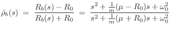
where
Bridge Transmittance
The bridge transmittance is the filter needed for the signal path from the vibrating string to the resonant acoustic body.
Since the bridge velocity equals the string endpoint velocity (a ``series'' connection), the velocity transmittance is simply
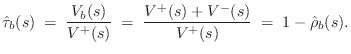
If the bridge is rigid, then its motion becomes a velocity input to the acoustic resonator. In principle, there are three such velocity inputs for each point along the bridge. However, it is typical in stringed instrument models to consider only the vertical transverse velocity on the string as significant, which results in one (vertical) driving velocity at the base of the bridge. In violin models (§9.6), the use of a ``sound post'' on one side of the bridge and ``bass bar'' on the other strongly suggests supporting a rocking motion along the bridge.
Digitizing Bridge Reflectance
Converting continuous-time transfer functions such as
![]() and
and
![]() to the digital domain is analogous to converting an analog
electrical filter to a corresponding digital filter--a problem which
has been well studied [343]. For this task, the
bilinear transform (§7.3.2) is a good choice. In
addition to preserving order and being free of aliasing, the bilinear
transform preserves the positive-real property of passive impedances
(§C.11.2).
to the digital domain is analogous to converting an analog
electrical filter to a corresponding digital filter--a problem which
has been well studied [343]. For this task, the
bilinear transform (§7.3.2) is a good choice. In
addition to preserving order and being free of aliasing, the bilinear
transform preserves the positive-real property of passive impedances
(§C.11.2).
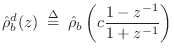
Digitizing
![]() via the bilinear transform (§7.3.2)
transform gives
via the bilinear transform (§7.3.2)
transform gives
A Two-Resonance Guitar Bridge
Now let's consider a two-resonance guitar bridge, as shown in Fig. 9.6.
![\includegraphics[width=\twidth]{eps/lguitarsynth2simp2}](http://www.dsprelated.com/josimages_new/pasp/img2001.png) |
Like all mechanical systems that don't ``slide away'' in response to a
constant applied input force, the bridge must ``look like a spring''
at zero frequency. Similarly, it is typical for systems to ``look
like a mass'' at very high frequencies, because the driving-point
typically has mass (unless the driver is spring-coupled by what seems
to be massless spring). This implies the driving point admittance
should have a zero at dc and a pole at infinity. If we neglect
losses, as frequency increases up from zero, the first thing we
encounter in the admittance is a pole (a ``resonance'' frequency at
which energy is readily accepted by the bridge from the strings). As
we pass the admittance peak going up in frequency, the phase switches
around from being near ![]() (``spring like'') to being closer to
(``spring like'') to being closer to
![]() (``mass like''). (Recall the graphical method for
calculating the phase response of a linear system
[449].) Below the first resonance, we may say that the system
is stiffness controlled (admittance phase
(``mass like''). (Recall the graphical method for
calculating the phase response of a linear system
[449].) Below the first resonance, we may say that the system
is stiffness controlled (admittance phase
![]() ),
while above the first resonance, we say it is mass controlled
(admittance phase
),
while above the first resonance, we say it is mass controlled
(admittance phase
![]() ). This qualitative description is
typical of any lightly damped, linear, dynamic system. As we proceed
up the
). This qualitative description is
typical of any lightly damped, linear, dynamic system. As we proceed
up the ![]() axis, we'll next encounter a near-zero, or
``anti-resonance,'' above which the system again appears ``stiffness
controlled,'' or spring-like, and so on in alternation to infinity.
The strict alternation of poles and zeros near the
axis, we'll next encounter a near-zero, or
``anti-resonance,'' above which the system again appears ``stiffness
controlled,'' or spring-like, and so on in alternation to infinity.
The strict alternation of poles and zeros near the ![]() axis is
required by the positive real property of all passive
admittances (§C.11.2).
axis is
required by the positive real property of all passive
admittances (§C.11.2).
Measured Guitar-Bridge Admittance
![\includegraphics[width=\twidth]{eps/lguitardata}](http://www.dsprelated.com/josimages_new/pasp/img2004.png) |
A measured driving-point admittance [269]
for a real guitar bridge is shown in Fig. 9.7. Note
that at very low frequencies, the phase information does not appear to
be bounded by ![]() as it must be for the admittance to be
positive real (passive). This indicates a poor signal-to-noise ratio
in the measurements at very low frequencies. This can be verified by
computing and plotting the coherence function between the
bridge input and output signals using multiple physical
measurements.10.5
as it must be for the admittance to be
positive real (passive). This indicates a poor signal-to-noise ratio
in the measurements at very low frequencies. This can be verified by
computing and plotting the coherence function between the
bridge input and output signals using multiple physical
measurements.10.5
Figures 9.8 and 9.9 show overlays of the admittance magnitudes and phases, and also the input-output coherence, for three separate measurements. A coherence of 1 means that all the measurements are identical, while a coherence less than 1 indicates variation from measurement to measurement, implying a low signal-to-noise ratio. As can be seen in the figures, at frequencies for which the coherence is very close to 1, successive measurements are strongly in agreement, and the data are reliable. Where the coherence drops below 1, successive measurements disagree, and the measured admittance is not even positive real at very low frequencies.
![\includegraphics[width=\twidth]{eps/lguitarcoh}](http://www.dsprelated.com/josimages_new/pasp/img2006.png) |
![\includegraphics[width=\twidth]{eps/lguitarphs}](http://www.dsprelated.com/josimages_new/pasp/img2007.png) |
Building a Synthetic Guitar Bridge Admittance
To construct a synthetic guitar bridge model, we can first measure empirically the admittance of a real guitar bridge, or we can work from measurements published in the literature, as shown in Fig. 9.7. Each peak in the admittance curve corresponds to a resonance in the guitar body that is well coupled to the strings via the bridge. Whether or not the corresponding vibrational mode radiates efficiently depends on the geometry of the vibrational mode, and how well it couples to the surrounding air. Thus, a complete bridge model requires not only a synthetic bridge admittance which determines the reflectance ``seen'' on the string, but also a separate filter which models the transmittance from the bridge to the outside air; the transmittance filter normally contains the same poles as the reflectance filter, but the zeros are different. Moreover, keep in mind that each string sees a slightly different reflectance and transmittance because it is located at a slightly different point relative to the guitar top plate; this changes the coupling coefficients to the various resonating modes to some extent. (We normally ignore this for simplicity and use the same bridge filters for all the strings.)
Finally, also keep in mind that each string excites the bridge in three dimensions. The two most important are the horizontal and vertical planes of vibration, corresponding to the two planes of transverse vibration on the string. The vertical plane is normal to the guitar top plate, while the horizontal plane is parallel to the top plate. Longitudinal waves also excite the bridge, and they can be important as well, especially in the piano. Since longitudinal waves are much faster in strings than transverse waves, the corresponding overtones in the sound are normally inharmonically related to the main (nearly harmonic) overtones set up by the transverse string vibrations.
The frequency, complex amplitude, and width of each peak in the measured admittance of a guitar bridge can be used to determine the parameters of a second-order digital resonator in a parallel bank of such resonators being used to model the bridge impedance. This is a variation on modal synthesis [5,299]. However, for the bridge model to be passive when attached to a string, its transfer function must be positive real, as discused previously. Since strings are very nearly lossless, passivity of the bridge model is actually quite critical in practice. If the bridge model is even slightly active at some frequency, it can either make the whole guitar model unstable, or it might objectionably lengthen the decay time of certain string overtones.
We will describe two methods of constructing passive ``bridge filters'' from measured modal parameters. The first is guaranteed to be positive real but has some drawbacks. The second method gives better results, but it has to be checked for passivity and possibly modified to give a positive real admittance. Both methods illustrate more generally applicable signal processing methods.
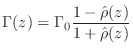
Passive Reflectance Synthesis--Method 1
The first method is based on constructing a passive reflectance
![]() having the desired poles, and then converting to an
admittance via the fundamental relation
having the desired poles, and then converting to an
admittance via the fundamental relation
As we saw in §C.11.1, every passive impedance corresponds
to a passive reflectance which is a Schur function (stable and having gain
not exceeding ![]() around the unit circle). Since damping is light in a
guitar bridge impedance (otherwise the strings would not vibrate very long,
and sustain is a highly prized feature of real guitars), we can expect the
bridge reflectance to be close to an allpass transfer function
around the unit circle). Since damping is light in a
guitar bridge impedance (otherwise the strings would not vibrate very long,
and sustain is a highly prized feature of real guitars), we can expect the
bridge reflectance to be close to an allpass transfer function ![]() .
.
It is well known that every allpass transfer function can be expressed as
We will then construct a Schur function as
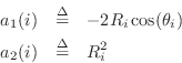
Recall that in every allpass filter with real coefficients, to every pole
at radius ![]() there corresponds a zero at radius
there corresponds a zero at radius ![]() .10.7
.10.7
Because the impedance is lightly damped, the poles and zeros of the
corresponding reflectance are close to the unit circle. This means that at
points along the unit circle between the poles, the poles and zeros tend to
cancel. It can be easily seen using the graphical method for computing the
phase of the frequency response that the pole-zero angles in the allpass
filter are very close to the resonance frequencies in the corresponding
passive impedance [429]. Furthermore, the distance of
the allpass poles to the unit circle controls the bandwidth of the
impedance peaks. Therefore, to a first approximation, we can treat the
allpass pole-angles as the same as those of the impedance pole angles, and
the pole radii in the allpass can be set to give the desired impedance peak
bandwidth. The zero-phase shaping filter ![]() gives the desired mode
height.
gives the desired mode
height.
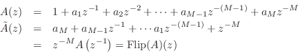
From the measured peak frequencies ![]() and bandwidths
and bandwidths ![]() in the guitar
bridge admittance, we may approximate the pole locations
in the guitar
bridge admittance, we may approximate the pole locations
![]() as
as
where ![]() is the sampling interval as usual. Next we construct the
allpass denominator as the product of elementary second-order sections:
is the sampling interval as usual. Next we construct the
allpass denominator as the product of elementary second-order sections:
Now that we've constructed a Schur function, a passive admittance can be computed using (9.2.1). While it is guaranteed to be positive real, the modal frequencies, bandwidths, and amplitudes are only indirectly controlled and therefore approximated. (Of course, this would provide a good initial guess for an iterative procedure which computes an optimal approximation directly.)
A simple example of a synthetic bridge constructed using this method
with ![]() and
and ![]() is shown in Fig.9.10.
is shown in Fig.9.10.
![\includegraphics[width=\twidth]{eps/lguitarsynth}](http://www.dsprelated.com/josimages_new/pasp/img2028.png)
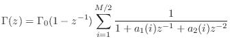
Passive Reflectance Synthesis--Method 2
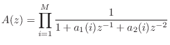
The second method is based on constructing a partial fraction expansion of the admittance directly:
A simple example of a synthetic bridge constructed using this method with is shown in Fig.9.11.
![\includegraphics[width=\twidth]{eps/lguitarsynth2}](http://www.dsprelated.com/josimages_new/pasp/img2031.png)
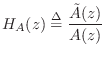
Matlab for Passive Reflectance Synthesis Method 1
fs = 8192;  % Sampling rate in Hz (small for display convenience)
fc = 300;   % Upper frequency to look at
nfft = 8192;% FFT size (spectral grid density)

nspec = nfft/2+1;
nc = round(nfft*fc/fs);
f = ([0:nc-1]/nfft)*fs;

% Measured guitar body resonances
F = [4.64 96.52 189.33 219.95]; % frequencies
B = [ 10   10     10     10  ]; % bandwidths

nsec = length(F);

R = exp(-pi*B/fs);     % Pole radii
theta = 2*pi*F/fs;     % Pole angles
poles = R .* exp(j*theta);
A1 = -2*R.*cos(theta);  % 2nd-order section coeff
A2 = R.*R;              % 2nd-order section coeff
denoms = [ones(size(A1)); A1; A2]'
A = [1,zeros(1,2*nsec)];
for i=1:nsec,
    % polynomial multiplication = FIR filtering:
    A = filter(denoms(i,:),1,A);
end;
Now A contains the (stable) denominator of the desired bridge admittance. We want now to construct a numerator which gives a positive-real result. We'll do this by first creating a passive reflectance and then computing the corresponding PR admittance.
g = 0.9;         % Uniform loss factor

B = g*fliplr(A); % Flip(A)/A = desired allpass

Badm = A - B;
Aadm = A + B;
Badm = Badm/Aadm(1); % Renormalize
Aadm = Aadm/Aadm(1);

% Plots

fr = freqz(Badm,Aadm,nfft,'whole');

nc = round(nfft*fc/fs);
spec = fr(1:nc);
f = ([0:nc-1]/nfft)*fs;
dbmag = db(spec);
phase = angle(spec)*180/pi;

subplot(2,1,1);
plot(f,dbmag); grid;
title('Synthetic Guitar Bridge Admittance');
ylabel('Magnitude (dB)');
subplot(2,1,2);

plot(f,phase); grid;
ylabel('Phase (degrees)');
xlabel('Frequency (Hz)');
Matlab for Passive Reflectance Synthesis Method 2
... as in Method 1 for poles ...

% Construct a resonator as a sum of arbitrary modes
% with unit residues, adding a near-zero at dc.

B = zeros(1,2*nsec+1);
impulse = [1,zeros(1,2*nsec)];
for i=1:nsec,
    % filter() does polynomial division here:
    B = B + filter(A,denoms(i,:),impulse);
end;

% add a near-zero at dc
B = filter([1 -0.995],1,B);

... as in Method 1 for display ...
Matrix Bridge Impedance
A passive matrix bridge admittance (e.g., taking all six strings of the guitar together) can be conveniently synthesized as a vector of positive-real scalar admittances multiplied by a positive definite matrix [25]. In [25], a dual-polarization guitar-string model is connected to a matrix reflectance computed from the matrix driving-point impedance at the bridge.
Body Modeling
As introduced in §8.7, the commuted synthesis technique involves commuting the LTI filter representing acoustic resonator (guitar body) with the string, so that the string is excited by the pluck response of the body in place of the plectrum directly. The techniques described in §8.8 can be used to build practical computational synthesis models of acoustic guitar bodies and the like [229].
Next Section:
String Excitation
Previous Section:
Electric Guitars


