


Acoustic Modeling with Digital Delay
Delay effects, such as phasing, flanging, chorus, and artificial reverberation, as well as digital waveguide models (Chapter 6), are built using delay lines, simple digital filter sections, and sometimes nonlinear elements and modulation. We will focus on these elements in the simpler context of delay effects before using them for sound synthesis.
Delay Lines
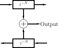
The delay line is an elementary functional unit which models acoustic propagation delay. It is a fundamental building block of both delay-effects processors and digital-waveguide synthesis models. The function of a delay line is to introduce a time delay between its input and output, as shown in Fig.2.1.
Let the input signal be denoted
![]() , and let the
delay-line length be
, and let the
delay-line length be ![]() samples. Then the output signal
samples. Then the output signal ![]() is
specified by the relation
is
specified by the relation
where
Before the digital era, delay lines were expensive and imprecise in
``analog'' form. For example, ``spring reverberators'' (common in
guitar amplifiers) use metal springs as analog delay lines; while
adequate for that purpose, they are highly dispersive and prone to
noise pick-up. Large delays require prohibitively long springs or
coils in analog implementations. In the digital domain, on the other
hand, delay by ![]() samples is trivially implemented, and non-integer
delays can be implemented using interpolation techniques, as discussed
later in §4.1.
samples is trivially implemented, and non-integer
delays can be implemented using interpolation techniques, as discussed
later in §4.1.
A Software Delay Line
In software, a delay line is often implemented using a circular
buffer. Let D denote an array of length ![]() . Then we can
implement the
. Then we can
implement the ![]() -sample delay line in the C programming
language as shown in Fig.2.2.
-sample delay line in the C programming
language as shown in Fig.2.2.
    /* delayline.c */
    static double D[M];  // initialized to zero
    static long ptr=0;   // read-write offset

    double delayline(double x)
    {
      double y = D[ptr];    // read operation
      D[ptr++] = x;         // write operation
      if (ptr >= M) { ptr -= M; } // wrap ptr
//    ptr %= M; // modulo-operator syntax
      return y;
    }
|
Delay lines of this type are typically used in digital reverberators and other acoustic simulators involving fixed propagation delays. Later, in Chapter 5, we will consider time-varying delay lengths.
Acoustic Wave Propagation Simulation
Delay lines can be used to simulate acoustic wave propagation. We start with the simplest case of a pure traveling wave, followed by the more general case of spherical waves. We then look at the details of a simple acoustic echo simulation using a delay line to model the difference in time-of-arrival between the direct and reflected signals.
Traveling Waves
In acoustic wave propagation, pure delays can be used to simulate traveling waves. A traveling wave is any kind of wave which propagates in a single direction with negligible change in shape. An important class of traveling waves is ``plane waves'' in air which create ``standing waves'' in rectangular enclosures such as ``shoebox'' shaped concert halls. Also, far away from any acoustic source (where ``far'' is defined as ``many wavelengths''), the direct sound emanating from any source can be well approximated as a plane wave, and thus as a traveling wave.
Another case in which plane waves dominate is the cylindrical bore, such as the bore of a clarinet or the straight tube segments of a trumpet. Additionally, the vocal tract is generally simulated using plane waves, though in this instance there is a higher degree of approximation error.
Transverse and longitudinal waves in a vibrating string, such as on a guitar, are also nearly perfect traveling waves, and they can be simulated to a very high degree of perceptual accuracy by approximating them as ideal, while implementing slight losses and dispersion once per period (i.e., at one particular point along the ``virtual string'').
In a conical bore, we find sections of spherical waves taking
the place of plane waves. However, they still ``travel'' like plane
waves, and we can still use a delay line to simulate their
propagation. The same applies to spherical waves created by a ``point
source.'' Spherical waves will be considered on
page ![]() .
.
Damped Traveling Waves
The delay line shown in Fig.2.1 on page ![]() can be used
to simulate any traveling wave, where the traveling wave must
propagate in one direction with a fixed waveshape. If a traveling
wave attenuates as it propagates, with the same attenuation
factor at each frequency, the attenuation can be simulated by a simple
scaling of the delay line output (or input), as shown in
Fig.2.3. This is perhaps the simplest example of
the important principle of lumping distributed losses at
discrete points. That is, it is not necessary to implement a small
attenuation
can be used
to simulate any traveling wave, where the traveling wave must
propagate in one direction with a fixed waveshape. If a traveling
wave attenuates as it propagates, with the same attenuation
factor at each frequency, the attenuation can be simulated by a simple
scaling of the delay line output (or input), as shown in
Fig.2.3. This is perhaps the simplest example of
the important principle of lumping distributed losses at
discrete points. That is, it is not necessary to implement a small
attenuation ![]() for each time-step of wave propagation; the same
result is obtained at the delay-line output if propagation is
``lossless'' within the delay line, and the total cumulative
attenuation
for each time-step of wave propagation; the same
result is obtained at the delay-line output if propagation is
``lossless'' within the delay line, and the total cumulative
attenuation ![]() is applied at the output. The input-output
simulation is exact, while the signal samples inside the delay line
are simulated with a slight gain error. If the internal signals are
needed later, they can be tapped out using correcting gains. For
example, the signal half way along the delay line can be tapped using
a coefficient of
is applied at the output. The input-output
simulation is exact, while the signal samples inside the delay line
are simulated with a slight gain error. If the internal signals are
needed later, they can be tapped out using correcting gains. For
example, the signal half way along the delay line can be tapped using
a coefficient of ![]() in order to make it an exact second output.
In summary, computational efficiency can often be greatly increased at
no cost to accuracy by lumping losses only at the outputs and points
of interaction with other simulations.
in order to make it an exact second output.
In summary, computational efficiency can often be greatly increased at
no cost to accuracy by lumping losses only at the outputs and points
of interaction with other simulations.
Modeling traveling-wave attenuation by a scale factor is only exact
physically when all frequency components decay at the same rate. For
accurate acoustic modeling, it is usually necessary to replace the
constant scale factor ![]() by a digital filter
by a digital filter ![]() which
implements frequency-dependent attenuation, as depicted in
Fig.2.4. In principle, a linear time-invariant (LTI) filter
can provide an independent attenuation factor at each frequency.
Section 2.3 addresses this case in more detail.
Frequency-dependent damping substitution will be used in artificial
reverberation design in §3.7.4.
which
implements frequency-dependent attenuation, as depicted in
Fig.2.4. In principle, a linear time-invariant (LTI) filter
can provide an independent attenuation factor at each frequency.
Section 2.3 addresses this case in more detail.
Frequency-dependent damping substitution will be used in artificial
reverberation design in §3.7.4.
Dispersive Traveling Waves
In many acoustic systems, such as piano strings
(§9.4.1,§C.6), wave propagation is also
significantly dispersive. A wave-propagation medium is said to
be dispersive if the speed of wave propagation is not the same at all
frequencies. As a result, a propagating wave shape will ``disperse''
(change shape) as its various frequency components travel at different
speeds. Dispersive propagation in one direction can be simulated
using a delay line in series with a nonlinear phase filter, as
indicated in Fig.2.5. If there is no damping, the filter
![]() must be all-pass [449], i.e.,
must be all-pass [449], i.e.,
![]() for
all
for
all
![]() .
.
Converting Propagation Distance to Delay Length
We may regard the delay-line memory itself as the fixed ``air'' which
propagates sound samples at a fixed speed ![]() (
(![]() meters per
second at
meters per
second at ![]() degrees Celsius and 1 atmosphere). The input signal
degrees Celsius and 1 atmosphere). The input signal
![]() can be associated with a sound source, and the output signal
can be associated with a sound source, and the output signal
![]() (see Fig.2.1 on page
(see Fig.2.1 on page ![]() ) can be associated with
the listening point. If the listening point is
) can be associated with
the listening point. If the listening point is ![]() meters away from
the source, then the delay line length
meters away from
the source, then the delay line length ![]() needs to be
needs to be
Spherical Waves from a Point Source
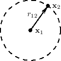
Acoustic theory tells us that a point source produces a spherical wave in an ideal isotropic (uniform) medium such as air. Furthermore, the sound from any radiating surface can be computed as the sum of spherical wave contributions from each point on the surface (including any relevant reflections). The Huygens-Fresnel principle explains wave propagation itself as the superposition of spherical waves generated at each point along a wavefront (see, e.g., [349, p. 175]). Thus, all linear acoustic wave propagation can be seen as a superposition of spherical traveling waves.
To a good first approximation, wave energy is conserved as it
propagates through the air. In a spherical pressure wave of radius
![]() , the energy of the wavefront is spread out over the spherical
surface area
, the energy of the wavefront is spread out over the spherical
surface area ![]() . Therefore, the energy per unit area of an
expanding spherical pressure wave decreases as
. Therefore, the energy per unit area of an
expanding spherical pressure wave decreases as ![]() . This is
called spherical spreading loss. It is also an example of an
inverse square law which is found repeatedly in the physics of
conserved quantities in three-dimensional space. Since energy is
proportional to amplitude squared, an inverse square law for energy
translates to a
. This is
called spherical spreading loss. It is also an example of an
inverse square law which is found repeatedly in the physics of
conserved quantities in three-dimensional space. Since energy is
proportional to amplitude squared, an inverse square law for energy
translates to a ![]() decay law for amplitude.
decay law for amplitude.
The sound-pressure amplitude of a traveling wave is proportional to
the square-root of its energy per unit area. Therefore, in a
spherical traveling wave, acoustic amplitude is proportional to ![]() ,
where
,
where ![]() is the radius of the sphere. In terms of Cartesian
coordinates, the amplitude
is the radius of the sphere. In terms of Cartesian
coordinates, the amplitude
![]() at the point
at the point
![]() due to a point source located at
due to a point source located at
![]() is given by
is given by
In summary, every point of a radiating sound source emits spherical
traveling waves in all directions which decay as ![]() , where
, where ![]() is
the distance from the source. The amplitude-decay by
is
the distance from the source. The amplitude-decay by ![]() can be
considered a consequence of energy conservation for propagating waves.
(The energy spreads out over the surface of an expanding sphere.) We
often visualize such waves as ``rays'' emanating from the source, and
we can simulate them as a delay line along with a
can be
considered a consequence of energy conservation for propagating waves.
(The energy spreads out over the surface of an expanding sphere.) We
often visualize such waves as ``rays'' emanating from the source, and
we can simulate them as a delay line along with a ![]() scaling
coefficient (see Fig.2.7). In contrast, since
plane waves propagate with no decay at all, each ``ray'' can be
considered lossless, and the simulation involves only a delay line
with no scale factor, as shown in Fig.2.1 on page
scaling
coefficient (see Fig.2.7). In contrast, since
plane waves propagate with no decay at all, each ``ray'' can be
considered lossless, and the simulation involves only a delay line
with no scale factor, as shown in Fig.2.1 on page ![]() .
.
Reflection of Spherical or Plane Waves
When a spreading spherical wave reaches a wall or other obstacle, it is either reflected or scattered. A wavefront is reflected when it impinges on a surface which is flat over at least a few wavelengths in each direction.3.1 Reflected wavefronts can be easily mapped using ray tracing, i.e., the reflected ray leaves at an angle to the surface equal to the angle of incidence (``law of reflection''). Wavefront reflection is also called specular reflection, especially when considering light waves.
A wave is scattered when it encounters a surface which has variations on the scale of the spatial wavelength. A scattering reflection is also called a diffuse reflection. As a special case, objects smaller than a wavelength yield a diffuse reflection which approaches a spherical wave as the object approaches zero volume. More generally, each point of a scatterer can be seen as emitting a new spherically spreading wavefront in response to the incoming wave--a decomposition known as Huygen's principle, as mentioned in the previous section. The same process happens in reflection, but the hemispheres emitted by each point of the flat reflecting surface combine to form a more organized wavefront which is the same as the incident wave but traveling in a new direction.
The distinction between specular and diffuse reflections is dependent
on frequency. Since sound travels approximately 1 foot per
millisecond, a cube 1 foot on each side will ``specularly reflect''
directed ``beams'' of sound energy above ![]() KHz, and will ``diffuse''
or scatter sound energy below
KHz, and will ``diffuse''
or scatter sound energy below ![]() KHz. A good concert hall, for
example, will have plenty of diffusion. As a general rule,
reverberation should be diffuse in order to avoid ``standing waves''
(isolated energetic modes). In other words, in reverberation, we wish
to spread the sound energy uniformly in both time and space, and we do
not want any specific spatial or temporal patterns in the
reverberation.
KHz. A good concert hall, for
example, will have plenty of diffusion. As a general rule,
reverberation should be diffuse in order to avoid ``standing waves''
(isolated energetic modes). In other words, in reverberation, we wish
to spread the sound energy uniformly in both time and space, and we do
not want any specific spatial or temporal patterns in the
reverberation.
An Acoustic Echo Simulator
An acoustic echo is one of the simplest acoustic modeling problems. Echoes occur when a sound arrives via more than one acoustic propagation path, as shown in Fig.2.8. We may hear a discrete echo, for example, if we clap our hands standing in front of a large flat wall outdoors, such as the side of a building. To be perceived as an echo, however, the reflection must arrive well after the direct signal (or previous echo).
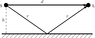 |
A common cause of echoes is ``multipath'' wave propagation, as
diagrammed in Fig.2.8. The acoustic source is denoted by `S',
the listener by `L', and they are at the same height ![]() meters
from a reflecting surface. The direct path is
meters
from a reflecting surface. The direct path is ![]() meters long, while
the length of the single reflection is
meters long, while
the length of the single reflection is ![]() meters. These quantities
are of course related by the Pythagorean theorem:
meters. These quantities
are of course related by the Pythagorean theorem:
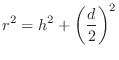
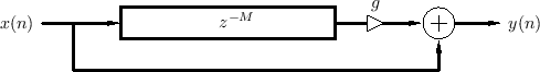
Figure 2.9 illustrates an echo simulator for the case of a direct signal and single echo, as shown in Fig.2.8. It is common practice to pull out and discard any common delay which affects all signals equally, since such a delay does not affect timbre; thus, the direct signal delay is not implemented at all in Fig.2.9. Similarly, it is not necessary to implement the attenuation of the direct signal due to propagation, since it is the relative amplitude of the direct signal and its echoes which affect timbre.
From the geometry in Fig.2.8, we see that the delay-line length in Fig.2.9 should be

Program for Acoustic Echo Simulation
The following main program (Fig.2.10) simulates a simple acoustic echo using the delayline function in Fig.2.2. It reads a sound file and writes a sound file containing a single, discrete echo at the specified delay. For simplicity, utilities from the free Synthesis Tool Kit (STK) (Version 4.2.x) are used for sound input/output [86].3.2
/* Acoustic echo simulator, main C++ program. Compatible with STK version 4.2.1. Usage: main inputsoundfile Writes main.wav as output soundfile */ #include "FileWvIn.h" /* STK soundfile input support */ #include "FileWvOut.h" /* STK soundfile output support */ static const int M = 20000; /* echo delay in samples */ static const int g = 0.8; /* relative gain factor */ #include "delayline.c" /* defined previously */ int main(int argc, char *argv[]) { long i; Stk::setSampleRate(FileRead(argv[1]).fileRate()); FileWvIn input(argv[1]); /* read input soundfile */ FileWvOut output("main"); /* creates main.wav */ long nsamps = input.getSize(); for (i=0;i<nsamps+M;i++) { StkFloat insamp = input.tick(); output.tick(insamp + g * delayline(insamp)); } } |
In summary, a delay line simulates the time delay associated
with wave propagation in a particular direction. Attenuation (e.g.,
by ![]() ) associated with ray propagation can of course be simulated
by multiplying the delay-line output by some constant
) associated with ray propagation can of course be simulated
by multiplying the delay-line output by some constant ![]() .
.
Lossy Acoustic Propagation
Attenuation of waves by spherical spreading, as described in
§2.2.5 above, is not the only source of amplitude decay
in a traveling wave. In air, there is always significant additional
loss caused by air absorption. Air absorption varies with
frequency, with high frequencies usually being more attenuated than
low frequencies, as discussed in §B.7.15. Wave
propagation in vibrating strings undergoes an analogous
absorption loss, as does the propagation of nearly every other kind of
wave in the physical world. To simulate such propagation losses, we
can use a delay line in series with a nondispersive filter, as
illustrated in §2.2.2 above. In practice, the desired attenuation
at each frequency becomes the desired magnitude frequency-response of
the filter in Fig.2.4, and filter-design software
(typically matlab) is used to compute the filter coefficients to
approximate the desired frequency response in some optimal way. The
phase response may be linear, minimum, or left unconstrained when
damping-filter dispersion is not considered harmful. There is
typically a frequency-dependent weighting on the approximation error
corresponding to audio perceptual importance (e.g., the weighting ![]() is a simple example that increases accuracy at low frequencies).
Some filter-design methods are summarized in §8.6.
is a simple example that increases accuracy at low frequencies).
Some filter-design methods are summarized in §8.6.
Exponentially Decaying Traveling Waves
Let
![]() denote the decay factor associated with
propagation of a plane wave over distance
denote the decay factor associated with
propagation of a plane wave over distance ![]() at frequency
at frequency
![]() rad/sec. For an ideal plane wave, there is no ``spreading
loss'' (attenuation by
rad/sec. For an ideal plane wave, there is no ``spreading
loss'' (attenuation by ![]() ). Under uniform conditions, the
amount of attenuation (in dB) is proportional to the distance
traveled; in other words, the attenuation factors for two successive
segments of a propagation path are multiplicative:
). Under uniform conditions, the
amount of attenuation (in dB) is proportional to the distance
traveled; in other words, the attenuation factors for two successive
segments of a propagation path are multiplicative:
Frequency-independent air absorption is easily modeled in an acoustic simulation by making the substitution
Frequency-Dependent Air-Absorption Filtering
More generally, frequency-dependent air absorption can be modeled using the substitution
For spherical waves, the loss due to spherical spreading is of the form
Dispersive Traveling Waves
In addition to frequency-dependent attenuation, LTI filters can provide a frequency-dependent delay. This can be used to simulate dispersive wave propagation, as introduced in §2.2.3.
Summary
Up to now, we have been concerned with the simulation of
traveling waves in linear, time-invariant (LTI) media.
The main example considered was wave propagation in air, but waves on
vibrating strings behave analogously. We saw that the point-to-point
propagation of a traveling plane wave in an LTI medium can be
simulated simply using only a delay line and an LTI
filter. The delay line simulates propagation delay, while the filter
further simulates (1) an independent attenuation factor at each
frequency by means of its amplitude response (e.g., to simulate air
absorption), and (2) a frequency-dependent propagation speed using its
phase response (to simulate dispersion). If there is additionally
spherical spreading loss, the amplitude may be further attenuated by
![]() , where
, where ![]() is the distance from the source. For more details
about the acoustics of plane waves and spherical waves, see, e.g.,
[318,349]. Appendix B contains a bit more about
elementary acoustics,
is the distance from the source. For more details
about the acoustics of plane waves and spherical waves, see, e.g.,
[318,349]. Appendix B contains a bit more about
elementary acoustics,
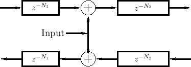
So far we have considered only traveling waves going in one direction. The next simplest case is 1D acoustic systems, such as vibrating strings and acoustic tubes, in which traveling waves may propagate in two directions. Such systems are simulated using a pair of delay lines called a digital waveguide.
Digital Waveguides
A (lossless) digital waveguide is defined as a
bidirectional delay line at some wave impedance ![]() [430,433].
Figure 2.11 illustrates one digital waveguide.
[430,433].
Figure 2.11 illustrates one digital waveguide.

As before, each delay line contains a sampled acoustic traveling wave.
However, since we now have a bidirectional delay line, we have
two traveling waves, one to the ``left'' and one to the
``right'', say. It has been known since 1747 [100] that
the vibration of an ideal string
can be described as the sum of two traveling waves going in opposite
directions. (See Appendix C for a mathematical derivation of this
important fact.) Thus, while a single delay line can model an
acoustic plane wave, a bidirectional delay line (a digital
waveguide) can model any one-dimensional linear acoustic system such
as a violin string, clarinet bore, flute pipe, trumpet-valve pipe, or
the like. Of course, in real acoustic strings and bores, the 1D
waveguides exhibit some loss and
dispersion3.4 so that we will need some filtering in
the waveguide to obtain an accurate physical model of such systems.
The wave impedance ![]() (derived in Chapter 6) is
needed for connecting digital waveguides to other physical simulations
(such as another digital waveguide or finite-difference model).
(derived in Chapter 6) is
needed for connecting digital waveguides to other physical simulations
(such as another digital waveguide or finite-difference model).
Physical Outputs
Physical variables (force, pressure, velocity, ...) are obtained by summing traveling-wave components, as shown in Fig.2.12, and more elaborated in Fig.2.13.
It is important to understand that the two traveling waves in a digital waveguide are now components of a more general acoustic vibration. The physical wave vibration is obtained by summing the left- and right-going traveling waves. A traveling wave by itself in one of the delay lines is no longer regarded as ``physical'' unless the signal in the opposite-going delay line is zero. Traveling waves are efficient for simulation, but they are not easily estimated from real-world measurements [476], except when the traveling-wave component in one direction can be arranged to be zero.
Note that traveling-wave components are not necessarily unique. For example, we can add a constant to the right-going wave and subtract the same constant from the left-going wave without altering the (physical) sum [263]. However, as derived in Appendix C (§C.3.6), 1D traveling-wave components are uniquely specified by two linearly independent physical variables along the waveguide, such as position and velocity (vibrating strings) or pressure and velocity (acoustic tubes).
Physical Inputs
A digital waveguide input signal corresponds to a disturbance of the 1D propagation medium. For example, a vibrating string is plucked or bowed by such an external disturbance. The result of the disturbance is wave propagation to the left and right of the input point. By physical symmetry, the amplitude of the left- and right-going propagating disturbances will normally be equal.3.5 If the disturbance superimposes with the waves already passing through at that point (an idealized case), then it is purely an additive input, as shown in Fig.2.14.
 |
Note that the superimposing input of Fig.2.14 is the graph-theoretic transpose of the ideal output shown in Fig.2.13. In other words, the superimposing input injects by means of two transposed taps. Transposed taps are discussed further in §2.5.2 below.
In practical reality, physical driving inputs do not merely superimpose with the current state of the driven system. Instead, there is normally some amount of interaction with the current system state (when it is nonzero), as discussed further in the next section. Note that there are similarly no ideal outputs as depicted in Fig.2.13. Real physical ouputs must present some kind of load on the system (energy must be extracted). Superimposing inputs and non-loading outputs are ideals that are often approximated in real-world systems. Of course, in the virtual world, they are no problem at all--in fact, they are usually easier to implement, and more efficient.
Interacting Physical Input
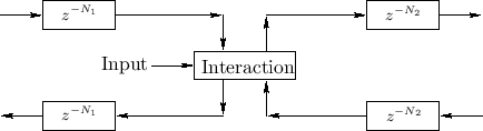
Figure 2.15 shows the general case of an input signal that interacts with the state of the system at one point along the waveguide. Since the interaction is physical, it only depends on the ``incoming state'' (traveling-wave components) and the driving input signal.
 |
A less general but commonly encountered case is shown in Fig.2.16. This case requires the ``outgoing disturbance'' to be distributed equally to the left and right, and it sums with the incoming waves to produce the outgoing waves.
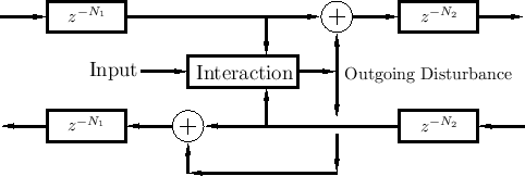
Figure 2.17 shows a further reduction in generality--also commonly encountered--in which the interaction depends only on the amplitude of the simulated physical variable (such as string velocity or displacement). The incoming amplitude is formed as the sum of the incoming traveling-wave components. We will encounter examples of this nature in later chapters (such as Chapter 9). It provides realistic models of physical excitations such as a guitar plectra, violin bows, and woodwind reeds.
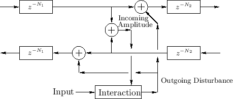 |
If an output signal is desired at this precise point, it can be computed as the incoming amplitude plus twice the outgoing disturbance signal (equivalent to summing the inputs of the two outgoing delay lines).
Note that the above examples all involve waveguide excitation at a single spatial point. While this can give a sufficiently good approximation to physical reality in many applications, one should also consider excitations that are spread out over multiple spatial samples (even just two).
We will develop the topic of digital waveguide modeling more systematically in Chapter 6 and Appendix C, among other places in this book. This section is intended only as a high-level preview and overview. For the next several chapters, we will restrict attention to normal signal processing structures in which signals may have physical units (such as acoustic pressure), and delay lines hold sampled acoustic waves propagating in one direction, but successive processing blocks do not ``load each other down'' or connect ``bidirectionally'' (as every truly physical interaction must, by Newton's third law3.6). Thus, when one processing block feeds a signal to a next block, an ``ideal output'' drives an ``ideal input''. This is typical in digital signal processing: Loading effects and return waves3.7 are neglected.3.8
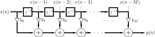
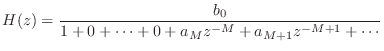
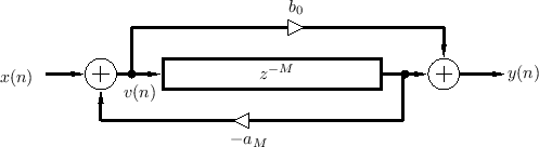
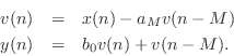
Tapped Delay Line (TDL)
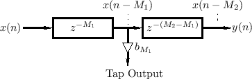
A tapped delay line (TDL) is a delay line with at least one ``tap''. A delay-line tap extracts a signal output from somewhere within the delay line, optionally scales it, and usually sums with other taps for form an output signal. A tap may be interpolating or non-interpolating. A non-interpolating tap extracts the signal at some fixed integer delay relative to the input. Thus, a tap implements a shorter delay line within a larger one, as shown in Fig.2.18.
Tapped delay lines efficiently simulate multiple echoes from the same source signal. As a result, they are extensively used in the field of artificial reverberation.
Example Tapped Delay Line
An example of a TDL with two internal taps is shown in
Fig.2.19. The total delay line length is ![]() samples, and the
internal taps are located at delays of
samples, and the
internal taps are located at delays of ![]() and
and ![]() samples,
respectively. The output signal is a linear combination of the input
signal
samples,
respectively. The output signal is a linear combination of the input
signal ![]() , the delay-line output
, the delay-line output ![]() , and the two tap
signals
, and the two tap
signals ![]() and
and ![]() .
.
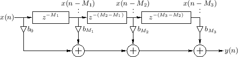
The difference equation of the TDL in Fig.2.19 is, by inspection,
Transposed Tapped Delay Line
In many applications, the transpose of a tapped delay line is desired, as shown in Fig.2.20, which is the transpose of the tapped delay line shown in Fig.2.19. A transposed TDL is obtained from a normal TDL by formal transposition of the system diagram. The transposition operation is also called flow-graph reversal [333, pp. 153-155]. A flow-graph is transposed by reversing all signal paths, which necessitates signal branchpoints becoming sums, and sums becoming branchpoints. For single-input, single-output systems, the transfer function is the same, but the input and output are interchanged. This ``flow-graph reversal theorem'' derives from Mason's gain formula for signal flow graphs. Transposition is used to convert direct-forms I and II of a digital filter to direct-forms III and IV, respectively [333].
TDL for Parallel Processing
When multiplies and additions can be performed in parallel, the
computational complexity of a tapped delay line is
![]() multiplies and
multiplies and
![]() additions, where
additions, where ![]() is the number of
taps. This computational complexity is achieved by arranging the
additions into a binary tree, as shown in Fig.2.21 for the
case
is the number of
taps. This computational complexity is achieved by arranging the
additions into a binary tree, as shown in Fig.2.21 for the
case ![]() .
.
 |
General Causal FIR Filters
The most general case--a TDL having a tap after every delay
element--is the general causal Finite Impulse Response (FIR)
filter, shown in Fig.2.22. It is restricted to be causal
because the output ![]() may not depend on ``future'' inputs
may not depend on ``future'' inputs
![]() ,
, ![]() , etc. The FIR filter is also called a
transversal filter. FIR filters are described in greater
detail in [449].
, etc. The FIR filter is also called a
transversal filter. FIR filters are described in greater
detail in [449].
The difference equation for the ![]() th-order FIR filter in Fig.2.22
is, by inspection,
th-order FIR filter in Fig.2.22
is, by inspection,
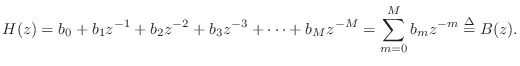
The STK class for implementing arbitrary direct-form FIR filters is called Fir. (There is also a class for IIR filters named Iir.) In Matlab and Octave, the built-in function filter is normally used.
Comb Filters
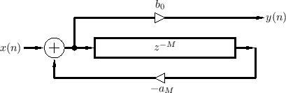
Comb filters are basic building blocks for digital audio effects. The acoustic echo simulation in Fig.2.9 is one instance of a comb filter. This section presents the two basic comb-filter types, feedforward and feedback, and gives a frequency-response analysis.
Feedforward Comb Filters
The feedforward comb filter is shown in Fig.2.23. The direct signal ``feeds forward'' around the delay line. The output is a linear combination of the direct and delayed signal.
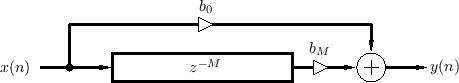
The ``difference equation'' [449] for the feedforward comb filter is
We see that the feedforward comb filter is a particular type of FIR filter. It is also a special case of a TDL.
Note that the feedforward comb filter can implement the echo simulator
of Fig.2.9 by setting ![]() and
and ![]() . Thus, it is is a
computational physical model of a single discrete echo. This
is one of the simplest examples of acoustic modeling using signal
processing elements. The feedforward comb filter models the
superposition of a ``direct signal''
. Thus, it is is a
computational physical model of a single discrete echo. This
is one of the simplest examples of acoustic modeling using signal
processing elements. The feedforward comb filter models the
superposition of a ``direct signal'' ![]() plus an attenuated,
delayed signal
plus an attenuated,
delayed signal
![]() , where the attenuation (by
, where the attenuation (by ![]() ) is
due to ``air absorption'' and/or spherical spreading losses, and the
delay is due to acoustic propagation over the distance
) is
due to ``air absorption'' and/or spherical spreading losses, and the
delay is due to acoustic propagation over the distance ![]() meters,
where
meters,
where ![]() is the sampling period in seconds, and
is the sampling period in seconds, and ![]() is sound speed.
In cases where the simulated propagation delay needs to be more
accurate than the nearest integer number of samples
is sound speed.
In cases where the simulated propagation delay needs to be more
accurate than the nearest integer number of samples ![]() , some kind of
delay-line interpolation needs to be used (the subject of
§4.1). Similarly, when air absorption needs to be
simulated more accurately, the constant attenuation factor
, some kind of
delay-line interpolation needs to be used (the subject of
§4.1). Similarly, when air absorption needs to be
simulated more accurately, the constant attenuation factor ![]() can
be replaced by a linear, time-invariant filter
can
be replaced by a linear, time-invariant filter ![]() giving a
different attenuation at every frequency. Due to the physics of air
absorption,
giving a
different attenuation at every frequency. Due to the physics of air
absorption, ![]() is generally lowpass in character [349, p. 560], [47,318].
is generally lowpass in character [349, p. 560], [47,318].
Feedback Comb Filters
The feedback comb filter uses feedback instead of a feedforward signal, as shown in Fig.2.24 (drawn in ``direct form 2'' [449]).
A difference equation describing the feedback comb filter can be written in ``direct form 1'' [449] as3.9
For stability, the feedback coefficient ![]() must be less than
must be less than
![]() in magnitude, i.e.,
in magnitude, i.e.,
![]() . Otherwise, if
. Otherwise, if
![]() ,
each echo will be louder than the previous echo, producing a
never-ending, growing series of echoes.
,
each echo will be louder than the previous echo, producing a
never-ending, growing series of echoes.
Sometimes the output signal is taken from the end of the delay line instead of the beginning, in which case the difference equation becomes
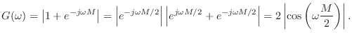
Feedforward Comb Filter Amplitude Response
Comb filters get their name from the ``comb-like'' appearance of their amplitude response (gain versus frequency), as shown in Figures 2.25, 2.26, and 2.27. For a review of frequency-domain analysis of digital filters, see, e.g., [449].
![\includegraphics[width=\twidth ]{eps/ffcfar}](http://www.dsprelated.com/josimages_new/pasp/img499.png) |
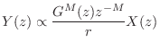
The transfer function of the feedforward comb filter Eq.![]() (2.2) is
(2.2) is
so that the amplitude response (gain versus frequency) is
This is plotted in Fig.2.25 for
Feedback Comb Filter Amplitude Response
Figure 2.26 shows a family of feedback-comb-filter amplitude responses, obtained using a selection of feedback coefficients.
![\includegraphics[width=\twidth ]{eps/fbcfar}](http://www.dsprelated.com/josimages_new/pasp/img505.png) |
Figure 2.27 shows a similar family obtained using negated feedback coefficients; the opposite sign of the feedback exchanges the peaks and valleys in the amplitude response.
![\includegraphics[width=\twidth ]{eps/fbcfiar}](http://www.dsprelated.com/josimages_new/pasp/img506.png) |
As introduced in §2.6.2 above, a class of feedback comb filters can be defined as any difference equation of the form
so that the amplitude response is
For ![]() , the feedback-comb amplitude response
reduces to
, the feedback-comb amplitude response
reduces to
Note that ![]() produces resonant peaks at
produces resonant peaks at
Filtered-Feedback Comb Filters
The filtered-feedback comb filter (FFBCF) uses filtered feedback instead of just a feedback gain.
Denoting the feedback-filter transfer function by ![]() , the
transfer function of the filtered-feedback comb filter can be written
as
, the
transfer function of the filtered-feedback comb filter can be written
as
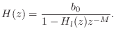
In §2.6.2 above, we mentioned the physical interpretation of a feedback-comb-filter as simulating a plane-wave bouncing back and forth between two walls. Inserting a lowpass filter in the feedback loop further simulates frequency dependent losses incurred during a propagation round-trip, as naturally occurs in real rooms.
The main physical sources of plane-wave attenuation are air absorption (§B.7.15) and the coefficient of absorption at each wall [349]. Additional ``losses'' for plane waves in real rooms occur due to scattering. (The plane wave hits something other than a wall and reflects off in many different directions.) A particular scatterer used in concert halls is textured wall surfaces. In ray-tracing simulations, reflections from such walls are typically modeled as having a specular and diffuse component. Generally speaking, wavelengths that are large compared with the ``grain size'' of the wall texture reflect specularly (with some attenuation due to any wall motion), while wavelengths on the order of or smaller than the texture grain size are scattered in various directions, contributing to the diffuse component of reflection.
The filtered-feedback comb filter has many applications in computer music. It was evidently first suggested for artificial reverberation by Schroeder [412, p. 223], and first implemented by Moorer [314]. (Reverberation applications are discussed further in §3.6.) In the physical interpretation [428,207] of the Karplus-Strong algorithm [236,233], the FFBCF can be regarded as a transfer-function physical-model of a vibrating string. In digital waveguide modeling of string and wind instruments, FFBCFs are typically derived routinely as a computationally optimized equivalent forms based on some initial waveguide model developed in terms of bidirectional delay-lines (``digital waveguides'') (see §6.10.1 for an example).
For stability, the amplitude-response of the feedback-filter
![]() must be less than
must be less than ![]() in magnitude at all frequencies, i.e.,
in magnitude at all frequencies, i.e.,
![]() .
.
Equivalence of Parallel Combs to TDLs
It is easy to show that the TDL of Fig.2.19 is equivalent to a
parallel combination of three feedforward comb filters, each as in
Fig.2.23. To see this, we simply add the three comb-filter transfer
functions of Eq.![]() (2.3) and equate coefficients:
(2.3) and equate coefficients:
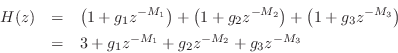
which implies
We see that parallel comb filters require more delay memory
(
![]() elements) than the corresponding TDL, which only
requires
elements) than the corresponding TDL, which only
requires
![]() elements.
elements.
Equivalence of Series Combs to TDLs
It is also straightforward to show that a series combination of feedforward comb filters produces a sparsely tapped delay line as well. Considering the case of two sections, we have
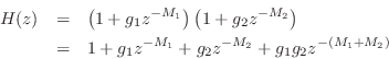
which yields
Time Varying Comb Filters
Comb filters can be changed slowly over time to produce the following digital audio ``effects'', among others:
Since all of these effects involve modulating delay length over time, and since time-varying delay lines typically require interpolation, these applications will be discussed after Chapter 5 which covers variable delay lines. For now, we will pursue what can be accomplished using fixed (time-invariant) delay lines. Perhaps the most important application is artificial reverberation, addressed in Chapter 3.
Feedback Delay Networks (FDN)
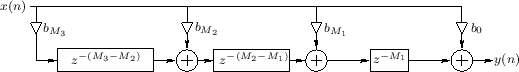
![\includegraphics[width=\twidth]{eps/FDNMIMO}](http://www.dsprelated.com/josimages_new/pasp/img529.png)
The FDN can be seen as a vector feedback comb filter,3.10obtained by replacing the delay line with a diagonal delay matrix
(defined in Eq.![]() (2.10) below), and replacing the feedback gain
(2.10) below), and replacing the feedback gain
![]() by the product of a diagonal matrix
by the product of a diagonal matrix
![]() times an orthogonal
matrix
times an orthogonal
matrix
![]() , as shown in
Fig.2.28 for
, as shown in
Fig.2.28 for ![]() . The time-update for this FDN can be written
as
. The time-update for this FDN can be written
as
![$\displaystyle \left[\begin{array}{c} x_1(n) \\ [2pt] x_2(n) \\ [2pt] x_3(n)\end...
...gin{array}{c} u_1(n) \\ [2pt] u_2(n) \\ [2pt] u_3(n)\end{array}\right] \protect$](http://www.dsprelated.com/josimages_new/pasp/img533.png)
with the outputs given by
![$\displaystyle \left[\begin{array}{c} y_1(n) \\ [2pt] y_2(n) \\ [2pt] y_3(n)\end...
...array}{c} x_1(n-M_1) \\ [2pt] x_2(n-M_2) \\ [2pt] x_3(n-M_3)\end{array}\right],$](http://www.dsprelated.com/josimages_new/pasp/img534.png) |
(3.7) |
or, in frequency-domain vector notation,
| (3.8) | |||
| (3.9) |
where
FDN and State Space Descriptions
When
![]() in Eq.
in Eq.![]() (2.10), the FDN (Fig.2.28)
reduces to a normal state-space model (§1.3.7),
(2.10), the FDN (Fig.2.28)
reduces to a normal state-space model (§1.3.7),
The matrix
to follow normal convention for state-space form.
Thus, an FDN can be viewed as a generalized state-space model for a
class of ![]() th-order linear systems--``generalized'' in the sense
that unit delays are replaced by arbitrary delays. This
correspondence is valuable for analysis because tools for state-space
analysis are well known and included in many software libraries such
as with matlab.
th-order linear systems--``generalized'' in the sense
that unit delays are replaced by arbitrary delays. This
correspondence is valuable for analysis because tools for state-space
analysis are well known and included in many software libraries such
as with matlab.
Single-Input, Single-Output (SISO) FDN
When there is only one input signal ![]() , the input vector
, the input vector
![]() in Fig.2.28 can be defined as the scalar input
in Fig.2.28 can be defined as the scalar input ![]() times a
vector of gains:
times a
vector of gains:
![\includegraphics[width=\twidth]{eps/FDNSISO}](http://www.dsprelated.com/josimages_new/pasp/img555.png)
Note that when
![]() , this system is capable of realizing
any transfer function of the form
, this system is capable of realizing
any transfer function of the form
The more general case shown in Fig.2.29 can be handled in one of
two ways: (1) the matrices
![]() can be augmented
to order
can be augmented
to order
![]() such that the three delay lines are replaced
by
such that the three delay lines are replaced
by ![]() unit-sample delays, or (2) ordinary state-space analysis
may be generalized to non-unit delays, yielding
unit-sample delays, or (2) ordinary state-space analysis
may be generalized to non-unit delays, yielding
![$\displaystyle \mathbf{D}(z) \isdef \left[\begin{array}{ccc} z^{-M_1} & 0 & 0\\ [2pt] 0 & z^{-M_2} & 0\\ [2pt] 0 & 0 & z^{-M_3} \end{array}\right]. \protect$](http://www.dsprelated.com/josimages_new/pasp/img539.png)
In FDN reverberation applications,
![]() , where
, where
![]() is an orthogonal matrix, for reasons addressed below, and
is an orthogonal matrix, for reasons addressed below, and
![]() is a
diagonal matrix of lowpass filters, each having gain bounded by 1. In
certain applications, the subset of orthogonal matrices known as
circulant matrices have advantages [385].
is a
diagonal matrix of lowpass filters, each having gain bounded by 1. In
certain applications, the subset of orthogonal matrices known as
circulant matrices have advantages [385].
FDN Stability
Stability of the FDN is assured when some norm [451] of
the state vector
![]() decreases over time when the input signal is
zero [220, ``Lyapunov stability theory'']. That is, a
sufficient condition for FDN stability is
decreases over time when the input signal is
zero [220, ``Lyapunov stability theory'']. That is, a
sufficient condition for FDN stability is
for all
![$\displaystyle \mathbf{x}(n+1) = \mathbf{A}\left[\begin{array}{c} x_1(n-M_1) \\ [2pt] x_2(n-M_2) \\ [2pt] x_3(n-M_3)\end{array}\right].
$](http://www.dsprelated.com/josimages_new/pasp/img567.png)
for all
The matrix norm corresponding to any vector norm
![]() may be defined for the matrix
may be defined for the matrix
![]() as
as
where
It can be shown [167] that the spectral norm of a matrix
![]() is given by the largest singular value of
is given by the largest singular value of
![]() (``
(``
![]() ''), and that this is equal to the
square-root of the largest eigenvalue of
''), and that this is equal to the
square-root of the largest eigenvalue of
![]() , where
, where
![]() denotes the matrix transpose of the real matrix
denotes the matrix transpose of the real matrix
![]() .3.11
.3.11
Since every orthogonal matrix
![]() has spectral norm
1,3.12 a wide variety of stable
feedback matrices can be parametrized as
has spectral norm
1,3.12 a wide variety of stable
feedback matrices can be parametrized as
![$\displaystyle {\bm \Gamma}= \left[ \begin{array}{cccc}
g_1 & 0 & \dots & 0\\
0...
...\\
0 & 0 & \dots & g_N
\end{array}\right], \quad \left\vert g_i\right\vert<1.
$](http://www.dsprelated.com/josimages_new/pasp/img587.png)
An alternative stability proof may be based on showing that an FDN is
a special case of a passive digital waveguide network (derived in
§C.15). This analysis reveals that the FDN is lossless if
and only if the feedback matrix
![]() has unit-modulus eigenvalues
and linearly independent eigenvectors.
has unit-modulus eigenvalues
and linearly independent eigenvectors.
Allpass Filters
The allpass filter is an important building block for digital audio signal processing systems. It is called ``allpass'' because all frequencies are ``passed'' in the same sense as in ``lowpass'', ``highpass'', and ``bandpass'' filters. In other words, the amplitude response of an allpass filter is 1 at each frequency, while the phase response (which determines the delay versus frequency) can be arbitrary.
In practice, a filter is often said to be allpass if the amplitude response is any nonzero constant. However, in this book, the term ``allpass'' refers to unity gain at each frequency.
In this section, we will first make an allpass filter by cascading a feedback comb-filter with a feedforward comb-filter. This structure, known as the Schroeder allpass comb filter, or simply the Schroeder allpass section, is used extensively in the fields of artificial reverberation and digital audio effects. Next we will look at creating allpass filters by nesting them; allpass filters are nested by replacing delay elements (which are allpass filters themselves) with arbitrary allpass filters. Finally, we will consider the general case, and characterize the set of all single-input, single-output allpass filters. The general case, including multi-input, multi-output (MIMO) allpass filters, is treated in [449, Appendix D].
Allpass from Two Combs
An allpass filter can be defined as any filter having a gain of
![]() at all frequencies (but typically different delays at different
frequencies).
at all frequencies (but typically different delays at different
frequencies).
It is well known that the series combination of a feedforward and feedback comb filter (having equal delays) creates an allpass filter when the feedforward coefficient is the negative of the feedback coefficient.
Figure 2.30 shows a combination feedforward/feedback comb filter structure which shares the same delay line.3.13 By inspection of Fig.2.30, the difference equation is
This can be recognized as a digital filter in direct form II
[449]. Thus, the system of Fig.2.30 can be interpreted as
the series combination of a feedback comb filter (Fig.2.24) taking
![]() to
to ![]() followed by a feedforward comb filter (Fig.2.23)
taking
followed by a feedforward comb filter (Fig.2.23)
taking ![]() to
to ![]() . By the commutativity of LTI systems, we can
interchange the order to get
. By the commutativity of LTI systems, we can
interchange the order to get
Substituting the right-hand side of the first equation above for
![]() in the second equation yields more simply
in the second equation yields more simply
This can be recognized as direct form I [449], which requires
The coefficient symbols ![]() and
and ![]() here have been chosen to
correspond to standard notation for the transfer function
here have been chosen to
correspond to standard notation for the transfer function

An allpass filter is obtained when
![]() , or, in the case
of real coefficients, when
, or, in the case
of real coefficients, when ![]() . To see this, let
. To see this, let
![]() . Then we have
. Then we have
Nested Allpass Filters
An interesting property of allpass filters is that they can be
nested [412,152,153].
That is, if ![]() and
and
![]() denote unity-gain allpass transfer functions, then both
denote unity-gain allpass transfer functions, then both
![]() and
and
![]() are allpass filters. A proof can be
based on the observation that, since
are allpass filters. A proof can be
based on the observation that, since
![]() ,
, ![]() can
be viewed as a conformal map
[326] which maps the unit circle in the
can
be viewed as a conformal map
[326] which maps the unit circle in the ![]() plane to itself;
therefore, the set of all such maps is closed under functional
composition. Nested allpass filters were proposed for use in artificial
reverberation by Schroeder [412, p. 222].
plane to itself;
therefore, the set of all such maps is closed under functional
composition. Nested allpass filters were proposed for use in artificial
reverberation by Schroeder [412, p. 222].
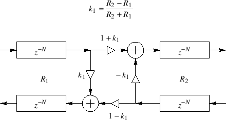
An important class of nested allpass filters is obtained by nesting first-order allpass filters of the form
![$\displaystyle H_2(z) \isdef S_1\left([z^{-1}S_2(z)]^{-1}\right) \isdef \frac{k_1+z^{-1}S_2(z)}{1+k_1z^{-1}S_2(z)}.
$](http://www.dsprelated.com/josimages_new/pasp/img609.png)
The equivalence of nested allpass filters to lattice filters has computational significance since it is well known that the two-multiply lattice sections can be replaced by one-multiply lattice sections [297,314].
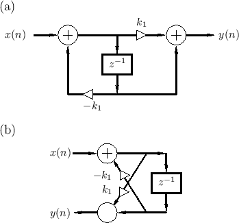 |
![\includegraphics[width=4.45in]{eps/aptwo}](http://www.dsprelated.com/josimages_new/pasp/img612.png) |
In summary, nested first-order allpass filters are equivalent to lattice filters made of two-multiply lattice sections. In §C.8.4, a one-multiply section is derived which is not only less expensive to implement in hardware, but it additionally has a direct interpretation as a physical model.
More General Allpass Filters
We have so far seen two types of allpass filters:
- The series combination of feedback and feedforward comb-filters is allpass when their delay lines are the same length and their feedback and feedforward coefficents are the same. An example is shown in Fig.2.30.
- Any delay element in an allpass filter can be replaced by an allpass filter to obtain a new (typically higher order) allpass filter. The special case of nested first-order allpass filters yielded the lattice digital filter structure of Fig.2.32.
Definition:
A linear, time-invariant filter ![]() is said to be
lossless if it preserves signal
energy for every input signal. That is, if the input signal is
is said to be
lossless if it preserves signal
energy for every input signal. That is, if the input signal is
![]() , and the output signal is
, and the output signal is
![]() , we must have
, we must have
Notice that only stable filters can be lossless since, otherwise,
![]() is generally infinite, even when
is generally infinite, even when
![]() is finite. We
further assume all filters are causal3.14 for
simplicity. It is straightforward to show the following:
is finite. We
further assume all filters are causal3.14 for
simplicity. It is straightforward to show the following:
It can be shown [449, Appendix C] that stable, linear,
time-invariant (LTI) filter transfer function ![]() is lossless if
and only if
is lossless if
and only if
Thus, ``lossless'' and ``unity-gain allpass'' are synonymous. For an
allpass filter with gain ![]() at each frequency, the energy gain of the
filter is
at each frequency, the energy gain of the
filter is ![]() for every input signal
for every input signal ![]() . Since we can describe
such a filter as an allpass times a constant gain, the term
``allpass'' will refer here to the case
. Since we can describe
such a filter as an allpass times a constant gain, the term
``allpass'' will refer here to the case ![]() .
.
Example Allpass Filters
- The simplest allpass filter is a unit-modulus gain
where

 can be any phase value. In the real case
can only be 0 or
can be any phase value. In the real case
can only be 0 or  , in which case
 .
.
- A lossless FIR filter can consist only of a single nonzero tap:
for some fixed integer
 , where is again some constant phase,
constrained to be 0 or in the real-filter case. Since we are
considering only causal filters here,
, where is again some constant phase,
constrained to be 0 or in the real-filter case. Since we are
considering only causal filters here,  . As a special case of
this example, a unit delay
. As a special case of
this example, a unit delay
 is a simple FIR allpass filter.
- The transfer function of every finite-order, causal,
lossless IIR digital filter (recursive allpass filter) can be written as
where,
 , and
, and
 . The polynomial
 can be obtained by reversing the order of the coefficients in
 and conjugating them. (The factor
  serves to restore
negative powers of
serves to restore
negative powers of  and hence causality.)
Gerzon Nested MIMO Allpass
An interesting generalization of the single-input, single-output Schroeder allpass filter (defined in §2.8.1) was proposed by Gerzon [157] for use in artificial reverberation systems.
The starting point can be the first-order allpass of Fig.2.31a on
page ![]() , or the allpass made from two comb-filters depicted
in Fig.2.30 on
page
, or the allpass made from two comb-filters depicted
in Fig.2.30 on
page ![]() .3.15In either case,
.3.15In either case,
- all signal paths are converted from scalars to vectors of dimension
 ,
,
- the delay element (or delay line) is replaced by an arbitrary
 unitary matrix frequency response.3.16
Let
![]() denote the
denote the ![]() input vector with components
input vector with components
![]() , and let
, and let
![]() denote
the corresponding vector of z transforms. Denote the
denote
the corresponding vector of z transforms. Denote the ![]() output
vector by
output
vector by
![]() . The resulting vector difference equation becomes,
in the frequency domain (cf. Eq.
. The resulting vector difference equation becomes,
in the frequency domain (cf. Eq.![]() (2.15))
(2.15))
Note that to avoid implementing
![]() twice,
twice,
![]() should
be realized in vector direct-form II, viz.,
should
be realized in vector direct-form II, viz.,

where ![]() denotes the unit-delay operator (
denotes the unit-delay operator (
![]() ).
).
To avoid a delay-free loop, the paraunitary matrix must include at
least one pure delay in every row, i.e.,
![]() where
where
![]() is paraunitary and causal.
is paraunitary and causal.
In [157], Gerzon suggested using
![]() of the form
of the form
![$\displaystyle \mathbf{D}(z) = \left[ \begin{array}{ccccc} z^{-m_1} & 0 & 0 & \d...
...ts & \ddots& \vdots\\ 0 & 0 & 0 & \dots & z^{-m_N} \end{array} \right] \protect$](http://www.dsprelated.com/josimages_new/pasp/img652.png)
is a diagonal matrix of pure delays, with the lengths
Gerzon further suggested replacing the feedback and feedforward gains
![]() by digital filters
by digital filters ![]() having an amplitude response
bounded by 1. In principle, this allows the network to be arbitrarily
different at each frequency.
having an amplitude response
bounded by 1. In principle, this allows the network to be arbitrarily
different at each frequency.
Gerzon's vector Schroeder allpass is used in the IRCAM Spatialisateur [218].
Allpass Digital Waveguide Networks
We now describe the class of multi-input, multi-output (MIMO) allpass filters which can be made using closed waveguide networks. We will see that feedback delay networks can be obtained as a special case.
Signal Scattering
The digital waveguide was introduced in §2.4. A basic fact from acoustics is that traveling waves only happen in a uniform medium. For a medium to be uniform, its wave impedance3.17must be constant. When a traveling wave encounters a change in the wave impedance, it will reflect, at least partially. If the reflection is not total, it will also partially transmit into the new impedance. This is called scattering of the traveling wave.
Let ![]() denote the constant impedance in some waveguide, such as a
stretched steel string or acoustic bore. Then signal scattering is
caused by a change in wave impedance from
denote the constant impedance in some waveguide, such as a
stretched steel string or acoustic bore. Then signal scattering is
caused by a change in wave impedance from ![]() to
to ![]() . We can
depict the partial reflection and transmission as shown in
Fig.2.33.
. We can
depict the partial reflection and transmission as shown in
Fig.2.33.
The computation of reflection and transmission in both directions, as shown in Fig.2.33 is called a scattering junction.
As derived in Appendix C, for force or pressure waves, the
reflection coefficient ![]() is given by
is given by
That is, the coefficient of reflection for a traveling pressure wave leaving impedance
For velocity traveling waves, the reflection coefficient is
just the negative of that for force/pressure waves, or ![]() (see
Appendix C).
(see
Appendix C).
Signal scattering is lossless, i.e., wave energy is neither
created nor destroyed. An implication of this is that the
transmission coefficient
for a traveling pressure wave leaving impedance ![]() and entering
impedance
and entering
impedance ![]() is given by
is given by
Digital Waveguide Networks
A Digital Waveguide Network (DWN) consists of any number of digital waveguides interconnected by scattering junctions. For example, when two digital waveguides are connected together at their endpoints, we obtain a two-port scattering junction as shown in Fig.2.33. When three or more waveguides are connected at a point, we obtain a multiport scattering junction, as discussed in §C.8. In other words, a digital waveguide network is formed whenever digital waveguides having arbitrary wave impedances are interconnected. Since DWNs are lossless, they provide a systematic means of building a very large class of MIMO allpass filters.
Consider the following question:
Under what conditions may I feed a signal from one point inside a given allpass filter to some other point (adding them) without altering signal energy at any frequency?In other words, how do we add feedback paths anywhere and everywhere, thereby maximizing the richness of the recursive feedback structure, while maintaining an overall allpass structure?
The digital waveguide approach to allpass design [430] answers this question by maintaining a physical interpretation for all delay elements in the system. Allpass filters are made out of lossless digital waveguides arranged in closed, energy conserving networks. See Appendix C for further discussion.
Next Section:
Artificial Reverberation
Previous Section:
Introduction to Physical Signal Models


