Acoustic Wave Propagation Simulation

Delay lines can be used to simulate acoustic wave propagation. We start with the simplest case of a pure traveling wave, followed by the more general case of spherical waves. We then look at the details of a simple acoustic echo simulation using a delay line to model the difference in time-of-arrival between the direct and reflected signals.

Traveling Waves

In acoustic wave propagation, pure delays can be used to simulate traveling waves. A traveling wave is any kind of wave which propagates in a single direction with negligible change in shape. An important class of traveling waves is ``plane waves'' in air which create ``standing waves'' in rectangular enclosures such as ``shoebox'' shaped concert halls. Also, far away from any acoustic source (where ``far'' is defined as ``many wavelengths''), the direct sound emanating from any source can be well approximated as a plane wave, and thus as a traveling wave.

Another case in which plane waves dominate is the cylindrical bore, such as the bore of a clarinet or the straight tube segments of a trumpet. Additionally, the vocal tract is generally simulated using plane waves, though in this instance there is a higher degree of approximation error.

Transverse and longitudinal waves in a vibrating string, such as on a guitar, are also nearly perfect traveling waves, and they can be simulated to a very high degree of perceptual accuracy by approximating them as ideal, while implementing slight losses and dispersion once per period (i.e., at one particular point along the ``virtual string'').

In a conical bore, we find sections of spherical waves taking the place of plane waves. However, they still ``travel'' like plane waves, and we can still use a delay line to simulate their propagation. The same applies to spherical waves created by a ``point source.'' Spherical waves will be considered on page .

Damped Traveling Waves

Figure 2.3: Damped traveling-wave simulator. In addition to propagation delay by samples, there is attenuation by .

The delay line shown in Fig.2.1 on page can be used to simulate any traveling wave, where the traveling wave must propagate in one direction with a fixed waveshape. If a traveling wave attenuates as it propagates, with the same attenuation factor at each frequency, the attenuation can be simulated by a simple scaling of the delay line output (or input), as shown in Fig.2.3. This is perhaps the simplest example of the important principle of lumping distributed losses at discrete points. That is, it is not necessary to implement a small attenuation for each time-step of wave propagation; the same result is obtained at the delay-line output if propagation is ``lossless'' within the delay line, and the total cumulative attenuation is applied at the output. The input-output simulation is exact, while the signal samples inside the delay line are simulated with a slight gain error. If the internal signals are needed later, they can be tapped out using correcting gains. For example, the signal half way along the delay line can be tapped using a coefficient of in order to make it an exact second output. In summary, computational efficiency can often be greatly increased at no cost to accuracy by lumping losses only at the outputs and points of interaction with other simulations.

Modeling traveling-wave attenuation by a scale factor is only exact physically when all frequency components decay at the same rate. For accurate acoustic modeling, it is usually necessary to replace the constant scale factor by a digital filter which implements frequency-dependent attenuation, as depicted in Fig.2.4. In principle, a linear time-invariant (LTI) filter can provide an independent attenuation factor at each frequency. Section 2.3 addresses this case in more detail. Frequency-dependent damping substitution will be used in artificial reverberation design in §3.7.4.

Figure 2.4: Damped traveling-wave simulator. In principle, the digital filter provides an arbitrary attenuation corresponding to one sample of wave propagation at each frequency. Physically, we must have for all .

Dispersive Traveling Waves

In many acoustic systems, such as piano strings (§9.4.1,§C.6), wave propagation is also significantly dispersive. A wave-propagation medium is said to be dispersive if the speed of wave propagation is not the same at all frequencies. As a result, a propagating wave shape will ``disperse'' (change shape) as its various frequency components travel at different speeds. Dispersive propagation in one direction can be simulated using a delay line in series with a nonlinear phase filter, as indicated in Fig.2.5. If there is no damping, the filter must be all-pass [449], i.e., for all .

Figure 2.5: Dispersive traveling-wave simulator. In principle, the digital filter provides an arbitrary nonnegative delay corresponding to one sample of wave propagation at each frequency.

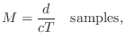
Converting Propagation Distance to Delay Length

We may regard the delay-line memory itself as the fixed ``air'' which propagates sound samples at a fixed speed ( meters per second at degrees Celsius and 1 atmosphere). The input signal can be associated with a sound source, and the output signal (see Fig.2.1 on page ) can be associated with the listening point. If the listening point is meters away from the source, then the delay line length needs to be

Spherical Waves from a Point Source

Acoustic theory tells us that a point source produces a spherical wave in an ideal isotropic (uniform) medium such as air. Furthermore, the sound from any radiating surface can be computed as the sum of spherical wave contributions from each point on the surface (including any relevant reflections). The Huygens-Fresnel principle explains wave propagation itself as the superposition of spherical waves generated at each point along a wavefront (see, e.g., [349, p. 175]). Thus, all linear acoustic wave propagation can be seen as a superposition of spherical traveling waves.

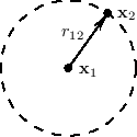
To a good first approximation, wave energy is conserved as it propagates through the air. In a spherical pressure wave of radius , the energy of the wavefront is spread out over the spherical surface area . Therefore, the energy per unit area of an expanding spherical pressure wave decreases as . This is called spherical spreading loss. It is also an example of an inverse square law which is found repeatedly in the physics of conserved quantities in three-dimensional space. Since energy is proportional to amplitude squared, an inverse square law for energy translates to a decay law for amplitude.

Figure 2.6: Geometry of wave propagation from a point source to a listening point .

The sound-pressure amplitude of a traveling wave is proportional to the square-root of its energy per unit area. Therefore, in a spherical traveling wave, acoustic amplitude is proportional to , where is the radius of the sphere. In terms of Cartesian coordinates, the amplitude at the point due to a point source located at is given by

In summary, every point of a radiating sound source emits spherical traveling waves in all directions which decay as , where is the distance from the source. The amplitude-decay by can be considered a consequence of energy conservation for propagating waves. (The energy spreads out over the surface of an expanding sphere.) We often visualize such waves as ``rays'' emanating from the source, and we can simulate them as a delay line along with a scaling coefficient (see Fig.2.7). In contrast, since plane waves propagate with no decay at all, each ``ray'' can be considered lossless, and the simulation involves only a delay line with no scale factor, as shown in Fig.2.1 on page .

Figure 2.7: Point-to-point spherical wave simulator. In addition to propagation delay, there is attenuation by .

Reflection of Spherical or Plane Waves

When a spreading spherical wave reaches a wall or other obstacle, it is either reflected or scattered. A wavefront is reflected when it impinges on a surface which is flat over at least a few wavelengths in each direction.^3.1 Reflected wavefronts can be easily mapped using ray tracing, i.e., the reflected ray leaves at an angle to the surface equal to the angle of incidence (``law of reflection''). Wavefront reflection is also called specular reflection, especially when considering light waves.

A wave is scattered when it encounters a surface which has variations on the scale of the spatial wavelength. A scattering reflection is also called a diffuse reflection. As a special case, objects smaller than a wavelength yield a diffuse reflection which approaches a spherical wave as the object approaches zero volume. More generally, each point of a scatterer can be seen as emitting a new spherically spreading wavefront in response to the incoming wave--a decomposition known as Huygen's principle, as mentioned in the previous section. The same process happens in reflection, but the hemispheres emitted by each point of the flat reflecting surface combine to form a more organized wavefront which is the same as the incident wave but traveling in a new direction.

The distinction between specular and diffuse reflections is dependent on frequency. Since sound travels approximately 1 foot per millisecond, a cube 1 foot on each side will ``specularly reflect'' directed ``beams'' of sound energy above KHz, and will ``diffuse'' or scatter sound energy below KHz. A good concert hall, for example, will have plenty of diffusion. As a general rule, reverberation should be diffuse in order to avoid ``standing waves'' (isolated energetic modes). In other words, in reverberation, we wish to spread the sound energy uniformly in both time and space, and we do not want any specific spatial or temporal patterns in the reverberation.

An Acoustic Echo Simulator

An acoustic echo is one of the simplest acoustic modeling problems. Echoes occur when a sound arrives via more than one acoustic propagation path, as shown in Fig.2.8. We may hear a discrete echo, for example, if we clap our hands standing in front of a large flat wall outdoors, such as the side of a building. To be perceived as an echo, however, the reflection must arrive well after the direct signal (or previous echo).

Figure 2.8: Geometry of an acoustic echo caused by ``multipath'' propagation. A direct signal and a ``floor bounce'' are received from the source S at the listening point L.

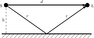A common cause of echoes is ``multipath'' wave propagation, as diagrammed in Fig.2.8. The acoustic source is denoted by `S', the listener by `L', and they are at the same height meters from a reflecting surface. The direct path is meters long, while the length of the single reflection is meters. These quantities are of course related by the Pythagorean theorem:

Figure 2.9: Acoustic echo simulation using a delay line, gain, and summer.

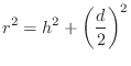
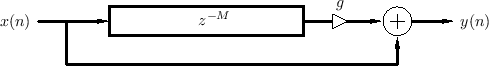
Figure 2.9 illustrates an echo simulator for the case of a direct signal and single echo, as shown in Fig.2.8. It is common practice to pull out and discard any common delay which affects all signals equally, since such a delay does not affect timbre; thus, the direct signal delay is not implemented at all in Fig.2.9. Similarly, it is not necessary to implement the attenuation of the direct signal due to propagation, since it is the relative amplitude of the direct signal and its echoes which affect timbre.

From the geometry in Fig.2.8, we see that the delay-line length in Fig.2.9 should be

Program for Acoustic Echo Simulation

The following main program (Fig.2.10) simulates a simple acoustic echo using the delayline function in Fig.2.2. It reads a sound file and writes a sound file containing a single, discrete echo at the specified delay. For simplicity, utilities from the free Synthesis Tool Kit (STK) (Version 4.2.x) are used for sound input/output [86].^3.2

/* Acoustic echo simulator, main C++ program.
   Compatible with STK version 4.2.1.
   Usage: main inputsoundfile
   Writes main.wav as output soundfile
 */

#include "FileWvIn.h"  /* STK soundfile input support */
#include "FileWvOut.h" /* STK soundfile output support */

static const int M = 20000; /* echo delay in samples */
static const int g = 0.8;   /* relative gain factor */

#include "delayline.c" /* defined previously */

int main(int argc, char *argv[])
{
  long i;
  Stk::setSampleRate(FileRead(argv[1]).fileRate());
  FileWvIn input(argv[1]);  /* read input soundfile */
  FileWvOut output("main"); /* creates main.wav */
  long nsamps = input.getSize();
  for (i=0;i<nsamps+M;i++)   {
    StkFloat insamp = input.tick();
    output.tick(insamp + g * delayline(insamp));
  }
}

In summary, a delay line simulates the time delay associated with wave propagation in a particular direction. Attenuation (e.g., by ) associated with ray propagation can of course be simulated by multiplying the delay-line output by some constant .

Sign in