


Artificial Reverberation
This chapter summarizes basic results in systems for artificial reverberation. Such systems make extensive use of tapped delay lines, comb filters, and allpass filters (described in the previous chapter).
The Reverberation Problem
Consider the requirements for acoustically simulating a concert hall or other listening space. Suppose we only need the response at one or more discrete listening points in space (``ears'') due to one or more discrete point sources of acoustic energy.
First, as discussed in §2.2, the direct signal
propagating from a sound source to a listener's ear can be simulated
using a single delay line in series with an attenuation scaling or
lowpass filter. Second, each sound ray arriving at the listening
point via one or more reflections can be simulated using a
delay-line and some scale factor (or filter). Two rays create a
feedforward comb filter, like the one in Fig.2.9 on
page ![]() . More generally, a tapped delay line
(Fig.2.19) can simulate many reflections. Each tap brings out one
echo at the appropriate delay and gain, and each tap can be
independently filtered to simulate air absorption and lossy
reflections. In principle, tapped delay lines can accurately simulate
any reverberant environment, because reverberation really does
consist of many paths of acoustic propagation from each source to each
listening point. As we will see, the only limitations of a tapped
delay line are (1) it is expensive computationally relative to
other techniques, (2) it handles only one ``point to point'' transfer
function, i.e., from one point-source to one ear,4.1 and (3) it should be changed when the source,
listener, or anything in the room moves.
. More generally, a tapped delay line
(Fig.2.19) can simulate many reflections. Each tap brings out one
echo at the appropriate delay and gain, and each tap can be
independently filtered to simulate air absorption and lossy
reflections. In principle, tapped delay lines can accurately simulate
any reverberant environment, because reverberation really does
consist of many paths of acoustic propagation from each source to each
listening point. As we will see, the only limitations of a tapped
delay line are (1) it is expensive computationally relative to
other techniques, (2) it handles only one ``point to point'' transfer
function, i.e., from one point-source to one ear,4.1 and (3) it should be changed when the source,
listener, or anything in the room moves.
Exact Reverb via Transfer-Function Modeling
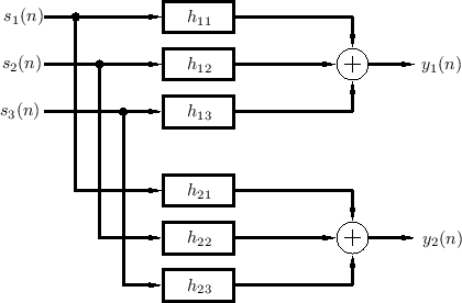
Figure 3.1 depicts the general reverberation scenario for three sources and one listener (two ears). In general, the filters should also include filtering by the pinnae of the ears, so that each echo can be perceived as coming from the correct angle of arrival in 3D space; in other words, at least some reverberant reflections should be spatialized so that they appear to come from their natural directions in 3D space [248]. Again, the filters change if anything changes in the listening space, including source or listener position. The artificial reverberation problem is then to implement some approximation of the system in Fig.3.1.
 |
In the frequency domain, it is convenient to express the input-output relationship in terms of the transfer-function matrix:
![$\displaystyle \left[\begin{array}{c} Y_1(z) \\ [2pt] Y_2(z) \end{array}\right] ...
...left[\begin{array}{c} S_1(z) \\ [2pt] S_2(z) \\ [2pt] S_3(z)\end{array}\right]
$](http://www.dsprelated.com/josimages_new/pasp/img663.png)
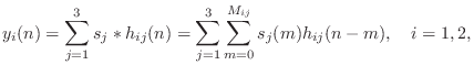
Denoting the impulse response of the filter from source ![]() to ear
to ear ![]() by
by ![]() , the two output signals in Fig.3.1 are computed by
six convolutions:
, the two output signals in Fig.3.1 are computed by
six convolutions:
Complexity of Exact Reverberation
For music, a typical reverberation time4.2is on the order of one second. Suppose we choose exactly one second for the reverberation time. At an audio sampling rate of 50 kHz, each filter in Fig.3.1 requires 50,000 multiplies and additions per sample, or 2.5 billion multiply-adds per second. Handling three sources and two listening points (ears), we reach 30 billion operations per second for the reverberator. This computational load would require at least 10 Pentium CPUs clocked at 3 Gigahertz, assuming they were doing nothing else, and assuming both a multiply and addition can be initiated each clock cycle, with no wait-states caused by the three required memory accesses (input, output, and filter coefficient). While these numbers can be improved using FFT convolution instead of direct convolution (at the price of introducing a throughput delay which can be a problem for real-time systems), it remains the case that exact implementation of all relevant point-to-point transfer functions in a reverberant space is very expensive computationally.
While a tapped delay line FIR filter can provide an accurate model for any point-to-point transfer function in a reverberant environment, it is rarely used for this purpose in practice because of the extremely high computational expense. While there are specialized commercial products that implement reverberation via direct convolution of the input signal with the impulse response, the great majority of artificial reverberation systems use other methods to synthesize the late reverb more economically.
Possibility of a Physical Reverb Model
One disadvantage of the point-to-point transfer function model depicted in Fig.3.1 is that some or all of the filters must change when anything moves. If instead we had a computational model of the whole acoustic space, sources and listeners could be moved as desired without affecting the underlying room simulation. Furthermore, we could use ``virtual dummy heads'' as listeners, complete with pinnae filters, so that all of the 3D directional aspects of reverberation could be captured in two extracted signals for the ears. Thus, there are compelling reasons to consider a full 3D model of a desired acoustic listening space.
Let us briefly estimate the computational requirements of a ``brute force'' acoustic simulation of a room. It is generally accepted that audio signals require a 20 kHz bandwidth. Since sound travels at about a foot per millisecond (see §B.7.14 for a more precise value), a 20 kHz sinusoid has a wavelength on the order of 1/20 feet, or about half an inch. Since, by elementary sampling theory, we must sample faster than twice the highest frequency present in the signal, we need ``grid points'' in our simulation separated by a quarter inch or less. At this grid density, simulating an ordinary 12'x12'x8' room in a home requires more than 100 million grid points. Using finite-difference (Appendix D) or waveguide-mesh techniques (§C.14,Appendix E) [518,396], the average grid point can be implemented as a multiply-free computation; however, since it has waves coming and going in six spatial directions, it requires on the order of 10 additions per sample. Thus, running such a room simulator at an audio sampling rate of 50 kHz requires on the order of 50 billion additions per second, which is comparable to the three-source, two-ear simulation of Fig.3.1. However, scaling up to a 100'x50'x20' concert hall requires more than 5 quadrillion operations per second. We may conclude, therefore, that a fine-grained physical model of a complete concert hall over the audio band is prohibitively expensive.
The remainder of this chapter will be concerned with ways of reducing computational complexity without sacrificing too much perceptual quality.
Perceptual Aspects of Reverberation
Artificial reverberation is an unusually interesting signal processing problem because, as discussed in the previous sections, the ``obvious'' methods based on physical modeling or input-output modeling are too expensive computationally for most applications. This leads to the question of what are the perceptually important aspects of reverberation, and how can these be provided by efficient computational structures.
Perception of Echo Density and Mode Density
The reverberation problem can be greatly simplified without
sacrificing perceptual quality. For example, it can be shown4.3that for typical rooms, the echo density increases as ![]() , where
, where ![]() is time. Therefore, beyond some time, the echo density is so great
that it can be modeled as some uniformly sampled stochastic process
without loss of perceptual fidelity. In particular, there is no need
to explicitly compute multiple echoes per sample of sound.
For smoothly decaying late reverb (the desired kind), an
appropriate random process sampled at the audio sampling rate will
sound equivalent perceptually.
is time. Therefore, beyond some time, the echo density is so great
that it can be modeled as some uniformly sampled stochastic process
without loss of perceptual fidelity. In particular, there is no need
to explicitly compute multiple echoes per sample of sound.
For smoothly decaying late reverb (the desired kind), an
appropriate random process sampled at the audio sampling rate will
sound equivalent perceptually.
Similarly, it can be shown4.4that the number of resonant modes in any given frequency band increases as frequency squared, so that above some frequency, the modes are so dense that they are perceptually equivalent to a random frequency response generated according to some statistics. In particular, there is no need to explicitly implement resonances so densely packed that the ear cannot hear them all.
In summary, we see that, based on limits of perception, the impulse response of a reverberant room can be divided into two segments. The first segment, called the early reflections, consists of the relatively sparse first echoes in the impulse response. The remainder, called the late reverberation, is so densely populated with echoes that it is best to characterize the response statistically in some way. Section 3.3 discusses methods for simulating early reflections in the reverberation impulse response.
Similarly, the frequency response of a reverberant room can be divided into two segments. The low-frequency interval consists of a relatively sparse distribution of resonant modes, while at higher frequencies the modes are packed so densely that they are best characterized statistically as a random frequency response with certain (regular) statistical properties. Section 3.4 describes methods for synthesizing hiqh quality late reverberation.
Perceptual Metrics for Ideal Reverberation
Some desirable controls for an artificial reverberator include [218]
-
 desired reverberation time at each frequency
 signal power gain at each frequency
 ``clarity'' = ratio of impulse-response energy in early reflections to that in the late reverb
 interaural correlation coefficient at left and right ears
The time to decay 60 dB (![]() ) is a classical objective parameter
used as a measure of perceived reverberation time. Classically,
) is a classical objective parameter
used as a measure of perceived reverberation time. Classically,
![]() was measured for the whole response. More recently
[216], it has become more common to design for a given
was measured for the whole response. More recently
[216], it has become more common to design for a given ![]() at more
than one frequency, e.g., one for low frequencies, another for high
frequencies, and interpolated values at intermediate frequencies.
Perceptual studies indicate that reverberation time should be
independently adjustable in at least three frequency bands
[217].
at more
than one frequency, e.g., one for low frequencies, another for high
frequencies, and interpolated values at intermediate frequencies.
Perceptual studies indicate that reverberation time should be
independently adjustable in at least three frequency bands
[217].
Energy Decay Curve
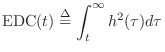
For measuring and defining reverberation time ![]() , Schroeder
introduced the so-called
energy decay curve (EDC) which is the tail integral of the squared impulse
response at time
, Schroeder
introduced the so-called
energy decay curve (EDC) which is the tail integral of the squared impulse
response at time ![]() :
:
Energy Decay Relief
The energy decay relief (EDR) is a time-frequency distribution which generalizes the EDC to multiple frequency bands [215]:
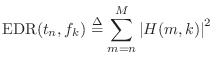
Thus,
![]() is the total amount of signal energy remaining
in the reverberator's impulse response at time
is the total amount of signal energy remaining
in the reverberator's impulse response at time ![]() in a frequency band centered
about
in a frequency band centered
about
![]() Hz, where
Hz, where ![]() denotes the FFT length.
denotes the FFT length.
The EDR of a violin-body impulse response is shown in Fig.3.2. For better correspondence with audio perception, the frequency axis is warped to the Bark frequency scale [459], and energy is summed within each Bark band (one critical band of hearing equals one Bark). A violin body can be regarded as a very small reverberant room, with correspondingly ``magnified'' spectral structure relative to reverberant rooms.
![\includegraphics[width=\twidth]{eps/bodyBEDR}](http://www.dsprelated.com/josimages_new/pasp/img693.png)
The EDR of the Boston Symphony Hall is displayed in [153, p. 96].
The EDR is used to measure partial overtone dampings from recordings of a vibrating string in §6.11.5.
Early Reflections
The ``early reflections'' portion of the impulse response of a reverberant environment is often taken to be the first 100ms or so [314]. However, for greater accuracy, it should be extended to the time at which the reverberation reaches its asymptotic statistical behavior.4.5
Since the early reflections are relatively sparse and span a relatively short time, they are often implemented using tapped delay lines (TDL).4.6
If the computation is affordable, it is best to spatialize the early reflections [248] so that they come from the right directions in 3D space. It is known [61] that the early reflections have a strong influence on spatial impression, i.e., the listener's perception of the listening-space shape.
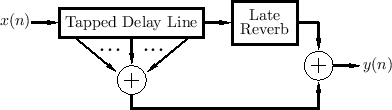
Figure 3.3 shows a general schematic of a reverberator with separate implementations of early and late reverberation. The taps on the TDL may include lowpass filtering for simulation of air absorption.
While the late reverb logically begins when the early reflections end, as implemented in Fig.3.3, it may be more cost-effective in practice to feed the ``late reverb'' unit from an earlier tap (or set of taps) from the TDL, thus overlapping them somewhat. This can help when the late reverberator needs time to build up to full density.
It is often the case that early reflections can be worked into the late-reverberation simulation. For example, usually there are long delay lines in which the input signal can be summed at various points, thereby implementing a transposed tapped delay line (see §2.5.2).
Good concert halls are observed to have to have stereo-recorded impulse responses that quickly ``lateralize'', with a smooth decay and overall duration of approximately 1.9 seconds [48].
Late Reverberation Approximations
Desired Qualities in Late Reverberation
From a perceptual standpoint, the main qualities desired of a good late-reverberation impulse response are
- a smooth (but not too smooth) decay, and
- a smooth (but not too regular) frequency response.
A smooth frequency response exhibits no large, isolated gaps or boosts. It is generally provided when the mode density is sufficiently large in the frequency domain, with the modes being spread out uniformly, as opposed to piling up in the same place or separated to form gaps. On the other hand, the modes should not be too regularly spaced, since this can produce audible periodicity in the time-domain impulse response.
An interesting experiment by Moorer [314] was to try exponentially decaying white noise as a late reverberation impulse response. This signal satisfies both smoothness criteria (time domain and frequency domain), and it sounds quite natural. However, since natural reverberation decays faster at high frequencies, it is better to say that the ideal late reverberation impulse response is exponentially decaying ``colored'' noise, with the high-frequency energy decaying faster than the low-frequency energy.
Schroeder's rule of thumb for echo density in the late reverb is 1000 echoes per second or more [417]. However, for impulsive sounds, 10,000 echoes per second or more may be necessary for a smooth response [217,153].
Schroeder Allpass Sections
Manfred Schroeder's original papers on the use of allpass filters for artificial reverberation [417,412,152,153] started a lively thread of research which continues to the present. For many years thereafter, digital reverberation algorithms were designed along the lines suggested by Schroeder using delay lines, comb filters, and allpass filters--elements described in Chapter 2. There was even special-purpose hardware developed to implement these structures efficiently in real time [393]. Today, these elements continue to serve as the basis for commercial devices for artificial reverberation and related effects [104]. They are also still typically used in software for artificial reverberation [86]. We will see some examples starting in §3.5 below.
Schroeder's suggested use of allpass filters was especially brilliant because there is nothing in nature to suggest them. Instead, he recognized the conceptual and practical utility of separating the coloration of reverberation from its duration and density aspects. While Schroeder's 1961 paper is entitled ``Colorless Artificial Reverberation,'' there is no such thing as colorless (exactly allpass) reverberation in the real world. However, it makes sense as an idealization of natural reverb. Colorless reverberation is an idealization only possible in the ``virtual world''.
In Schroeder's original work, and in much work which followed, allpass filters are arranged in series, as shown in Fig.3.4.
 |
Each allpass can be thought of as expanding each nonzero input sample from the previous stage into an entire infinite allpass impulse response. For this reason, Schroeder allpass sections are sometimes called impulse expanders [483] or impulse diffusers. While not a physical model of diffuse reflection, single reflections are expanded into many reflections, which is qualitatively what is desired.
Another interesting interpretation of a Schroeder allpass section is as a digital waveguide model of the driving-point impedance of an ideal string (or cylindrical acoustic tube) which is reflectively terminated at a real impedance. That is, if the input signal is regarded as samples of a physical velocity, then the output signal is proportional to samples of the corresponding force (or pressure) at the same physical point. The delay line contains traveling-wave samples; the first half corresponds to traveling waves heading toward the far end of the string (or tube), while the second half holds traveling-wave samples coming back the other way toward the driving point. For the mathematical details of this interpretation, see Appendix C.
Nested Allpass Filters
Another common method for increasing the density of an allpass impulse
response is to nest two or more allpass filters, as described
in §2.8.2 and shown in Fig.2.32 on page ![]() . In
general, a nested allpass filter is created when one or more of its
delay elements is replaced by another allpass filter. As we saw in
§2.8.2, first-order nested allpass filters are equivalent to
lattice filters. This equivalence implies that any order
. In
general, a nested allpass filter is created when one or more of its
delay elements is replaced by another allpass filter. As we saw in
§2.8.2, first-order nested allpass filters are equivalent to
lattice filters. This equivalence implies that any order ![]() transfer function (any
transfer function (any ![]() poles and zeros)
may be obtained from a linear combination of the
delay elements of nested first-order allpass filters, since this is a
known property of the lattice filter [297].
poles and zeros)
may be obtained from a linear combination of the
delay elements of nested first-order allpass filters, since this is a
known property of the lattice filter [297].
In general, any delay-element or delay-line inside a stable allpass-filter can be replaced with any stable allpass-filter, and the result will be a stable allpass.
Schroeder Reverberators
The subject of artificial reverberation was initiated in the early 1960s by Manfred Schroeder [417,412]. Early Schroeder reverberators consisted of the following elements [412]:
- A series connection of several allpass filters
- A parallel bank of feedback comb filters
- A mixing matrix
![\includegraphics[width=\twidth]{eps/jcrevmus10}](http://www.dsprelated.com/josimages_new/pasp/img706.png) |
An example is shown in Fig.3.5, where, in that figure,
denotes a Schroeder allpass section with delay length
denotes a feedback comb filter with delay length
![$\displaystyle \eqsp \left[\begin{array}{rrrr}
1 & 1 & 1 & 1 \\ [2pt]
-1 & -1 & -1 & -1 \\ [2pt]
-1 & 1 & -1 & 1 \\ [2pt]
1 & -1 & 1 & -1
\end{array}\right]
$](http://www.dsprelated.com/josimages_new/pasp/img709.png)
|

|
As discussed above in §3.4.2, the allpass filters provide ``colorless'' high-density echoes in the late impulse response of the reverberator [417]. These allpass filters may also be referred to as diffusers. While allpass filters are ``colorless'' in theory, perceptually, their impulse responses are only colorless when they are extremely short (less than 10 ms or so). Longer allpass impulse responses sound similar to feedback comb-filters. For steady-state tones, however, such as sinusoids, the allpass property gives the same gain at every frequency, unlike comb filters.
Schroeder [412, p. 221] suggests a progression of allpass delay-line lengths close to
The parallel comb-filter bank is intended to give a psychoacoustically appropriate fluctuation in the reverberator frequency response. As discussed in Chapter 2 (§2.6.2), a feedback comb filter can simulate a pair of parallel walls, so one could choose the delay-line length in each comb filter to be the number of samples it takes for a plane wave to propagate from one wall to the opposite wall and back. However, in his original paper [412], Schroeder describes a more psychoacoustically motivated approach:
``There are about 15 large response peaks in every 100 cps [Hz] interval for a room with 1 sec reverberation time. Thus, one might hope that if an artificial reverberator has a comparable number of response peaks it might sound just as good as a real room. We have been able to confirm this expectation by subjective evaluations of the responses of reverberators consisting of several comb filters ... connected in parallel. For a delay of 0.04 sec, the number of response peaks per 100 cps [Hz] is 4. Thus, between 3 and 4 comb filters in parallel ... with incommensurate delays, are required to approximate the number of peaks in the frequency reponse of a room having a reverberation time of T[60] = 1 sec. Also, the open loop gain of the comb filters should not exceed about 0.85 or -1.4 dB to keep the response fluctuations from being excessive.''Thus, one may choose the comb-filter delay-line lengths more or less arbitrarily, and then use enough of them in parallel (with mutually prime delay-line lengths) to achieve a perceptually adequate fluctuation density in the frequency-response magnitude. In [412], four such delays are chosen between 30 and 45 ms, and the corresponding feedback coefficients
The delay lengths shown in Fig.3.7 were optimized by ear by John
Chowning (and perhaps others at CCRMA) for an audio sampling rate of
![]() kHz.
kHz.
Finally, for multichannel listening, Schroeder suggested [412] a mixing matrix at the reverberator output. The goal of the mixing matrix is to bring out any number of uncorrelated audio channels of reverberation (for any number of output speakers) [153, p. 111-112].
Example Schroeder Reverberators
Additional example Schroeder Reverberators, drawn from CCRMA software listings, are shown in Figures 3.6 and 3.7. The notation used in the figures is explained above in Equations (3.2-3.3).
![\includegraphics[width=\twidth]{eps/satrev}](http://www.dsprelated.com/josimages_new/pasp/img719.png) |
![\includegraphics[width=\twidth]{eps/jcrev}](http://www.dsprelated.com/josimages_new/pasp/img720.png) |
A software musical instrument using one of these reverberators simply adds its output, suitably scaled, to the real-time variable RevIn (the global reverberator input sample at the current time). In both examples, we again see three Schroeder allpass filters in series (Schroeder suggested five, as disussed above).
The rather small reverberator of Fig.3.6 is thought to have been used in John Chowning's often-heard FM-brass canon sound examples.4.8Like the more computationally expensive four-channel-audio example in Fig.3.5, it is designed for a 25 kHz sampling rate. Its ``mixing matrix'' is simply a negation of the right stereo channel.
In addition to the allpass chain in Figures 3.6 and 3.7, there is a parallel bank of four feedback comb filters. Since all of the filters are linear and time-invariant [449], the series allpass chain can go either before or after the parallel comb-filter bank. Unlike the allpass filters, the comb filters have an irregular magnitude frequency response, and they can be considered a simulation of four specific echo sequences. The delay lengths in these comb filters may be used to adjust the illusion of ``room size'', although if they are shortened, there should be more of them in parallel, according to Schroeder's quote above.
In Fig.3.7, the reverbator output signal RevOut is fed
to the four audio output channels via four delay lines. These delay
lengths are specified relative to the sampling rate ![]() .4.9 Output delay lines can substitute for or supplement
a mixing matrix as a means for decorrelating the reverberation
output channels (to minimize reverberation imaging between
speakers). In this particular case, however, the delays are evidently
not optimized for decorrelation. Also, for purposes of decorrelation,
the shortest delay can be subtracted from the other three and its
corresponding delay-line eliminated.
.4.9 Output delay lines can substitute for or supplement
a mixing matrix as a means for decorrelating the reverberation
output channels (to minimize reverberation imaging between
speakers). In this particular case, however, the delays are evidently
not optimized for decorrelation. Also, for purposes of decorrelation,
the shortest delay can be subtracted from the other three and its
corresponding delay-line eliminated.
A Schroeder reverberator along the above lines may be found in the Synthesis Tool Kit (STK) [86]. See files JCRev.cpp and JCRev.h.
The reverberators shown in Figures 3.5 and 3.6 above are included in the Faust distribution. See functions jcrev, satrev, and reverb_demo in the effect.lib library. While these Schroeder reverberators are quite small by today's standards, they are well tuned for their size. More commonly used today is freeverb (included in the examples directory of the Faust distribution as freeverb.dsp), discussed next.
Freeverb
A more recently developed Schroeder reverberator is ``Freeverb'' -- a public domain C++ program by ``Jezar at Dreampoint'' used extensively in the free-software world. It uses four Schroeder allpasses in series and eight parallel Schroeder-Moorer filtered-feedback comb-filters (§2.6.5) for each audio channel, and is said to be especially well tuned.
![\includegraphics[width=\twidth]{eps/freeverb}](http://www.dsprelated.com/josimages_new/pasp/img724.png) |
Figure 3.8 shows the default signal-processing settings for the Freeverb left stereo channel. Processing for the right channel is obtained by adding an integer to each of the twelve delay-line lengths. This integer is called stereospread, and its default value is 23. (See the file tuning.h for all constants and default values used by Freeverb.) Different software distributions may include slightly different default values in tuning.h. The values in Fig.3.8 were found in the ladspa-cmt-plugins package (``Computer Music Toolkit'') which is included in the Planet CCRMA distribution, and which is based on the June 2000 version of Freeverb, as of this writing. There are at least six more instances of Freeverb in the Planet CCRMA distribution alone.4.10
Freeverb Main Loop
The C++ code for the main processing loop of Freeverb is shown in Fig.3.9. Notice that it sums the two stereo input channels to create a mono signal that is fed to the reverberator, which then computes a stereo output signal.
void revmodel::processreplace(float *inputL, float *inputR,
  float *outputL, float *outputR, long numsamples, int skip)
{
  float outL,outR,input;
  int i;

  while(numsamples-- > 0)
    {
      outL = outR = 0;
      input = (*inputL + *inputR) * gain;

      // Accumulate comb filters in parallel
      for(i=0; i<numcombs; i++) {
        outL += combL[i].process(input);
        outR += combR[i].process(input);
      }

      // Feed through allpasses in series
      for(i=0; i<numallpasses; i++) {
        outL = allpassL[i].process(outL);
        outR = allpassR[i].process(outR);
      }

      // Calculate output REPLACING anything already there
      *outputL = outL*wet1 + outR*wet2 + *inputL*dry;
      *outputR = outR*wet1 + outL*wet2 + *inputR*dry;

      // Increment sample pointers, allowing for interleave
      // (if any)
      inputL += skip; // For stereo buffers, skip = 2
      inputR += skip;
      outputL += skip;
      outputR += skip;
    }
}
|
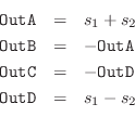
From the code in Fig.3.9, we see that the left and right reverberator output channels outL and outR are combined with the left and right input channels inputL and inputR as follows:
![$\displaystyle \left[\begin{array}{c} \texttt{outputL} \\ [2pt] \texttt{outputR}...
...\left[\begin{array}{c} \texttt{outL} \\ [2pt] \texttt{outR} \end{array}\right]
$](http://www.dsprelated.com/josimages_new/pasp/img725.png)
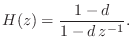
Lowpass-Feedback Comb Filter
Inspection of comb.h in the Freeverb source shows that Freeverb's ``comb'' filter is more specifically a lowpass-feedback-comb filter (LBCF4.11--§2.6.5). It is constructed using a delay line whose output is lowpass-filtered and summed with the delay-line's input. The particular lowpass used in Freeverb is a unity-gain one-pole lowpass having the transfer function
In Freeverb's comb section (comb.h and
comb.cpp), the ``damping'' ![]() is set initially to
is set initially to
Increasing the roomsize parameter (typically brought out to a
GUI slider) increases ![]() and hence the reverberation time. Since
and hence the reverberation time. Since
![]() is required for dc stability, the roomsize must be less
than 1.0714, and so the GUI slider max is typically 1 (
is required for dc stability, the roomsize must be less
than 1.0714, and so the GUI slider max is typically 1 (![]() ).
).
The feedback variable ![]() mainly determines reverberation
time at low-frequencies at which the feedback lowpass has negligible
effect. The feedback lowpass causes the reverberation time to
decrease with frequency, which is natural. At very high
frequencies--those for which the lowpass gain times
mainly determines reverberation
time at low-frequencies at which the feedback lowpass has negligible
effect. The feedback lowpass causes the reverberation time to
decrease with frequency, which is natural. At very high
frequencies--those for which the lowpass gain times ![]() is much less
than 0.5--the reverberation time becomes dominated by the diffusion
allpass filters (which have a fixed feedback coefficient of
is much less
than 0.5--the reverberation time becomes dominated by the diffusion
allpass filters (which have a fixed feedback coefficient of ![]() ).
Thus, in Freeverb, the ``room size'' parameter can be interpreted as
setting the low-frequency T60 (time to decay 60 dB), while the
``damping'' parameter controls how rapidly T60 shortens as a function
of increasing frequency. A lower-limit on T60 is given by the four
diffusion allpass filters.
).
Thus, in Freeverb, the ``room size'' parameter can be interpreted as
setting the low-frequency T60 (time to decay 60 dB), while the
``damping'' parameter controls how rapidly T60 shortens as a function
of increasing frequency. A lower-limit on T60 is given by the four
diffusion allpass filters.
In terms of the physical interpretation of the filtered-feedback comb-filter discussed in §2.6.5, Freeverb's roomsize parameter can be interpreted as the square-root of the low-frequency reflection-coefficient of each wall. That is, when a planewave bounces back and forth between two walls, the attenuation coefficient is roomsize after one round trip (two wall reflections). Therefore, a better name in this interpretation would be liveness or reflectivity. Since the round-trip delay is given in samples by the delay-line length, changing the roomsize requires changing the delay-line lengths in this interpretation.
Freeverb Allpass Approximation
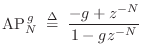
In Eq.![]() (3.2) we defined the allpass notation
(3.2) we defined the allpass notation
![]() by
by
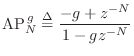

![\begin{eqnarray*}
\hbox{FBCF}_{N}^{\,g} &\isdef & \frac{1}{1 - g\,z^{-N}}\\ [5pt]
\hbox{FFCF}_{N}^{\,-1,1+g} &\isdef & -1 + (1+g)z^{-N}.
\end{eqnarray*}](http://www.dsprelated.com/josimages_new/pasp/img742.png)
A true allpass is obtained only for
![]() (reciprocal of the ``golden ratio''). The default value used in
Freeverb (see revmodel.cpp) is
(reciprocal of the ``golden ratio''). The default value used in
Freeverb (see revmodel.cpp) is ![]() . A detailed discussion
of feedforward and feedback comb filters appears
in §2.6, and corresponding Schroeder allpass filters are
described in §2.8.
. A detailed discussion
of feedforward and feedback comb filters appears
in §2.6, and corresponding Schroeder allpass filters are
described in §2.8.
Conclusions
Since Freeverb is a Schroeder-Moorer reverberator, and such reverbs have been around since the 1970s, its relatively recent success underscores the value of careful parameter tuning (typically by ear, but automatic optimizations are possible).
The idea of synthesizing right-channel processing from left-channel processing to obtain ``stereo spreading'' by enlarging all the delay lines by a fixed amount appears to have been introduced by Freeverb.
FDN Reverberation
Feedback Delay Networks (FDN) were introduced earlier in §2.7.
An example is shown in Fig.2.29 on page ![]() . After a
brief historical summary, this section will cover some practical
considerations for the use of FDNs as reverberators.
. After a
brief historical summary, this section will cover some practical
considerations for the use of FDNs as reverberators.
History of FDNs for Artificial Reverberation
Feedback delay networks were first suggested for artificial reverberation by Gerzon [156], who proposed an ``orthogonal matrix feedback reverberation unit''. He noted that individual feedback comb filters yielded poor quality, but that several such filters could sound good when cross-coupled. An ``orthogonal matrix feedback'' around a parallel bank of delay lines was suggested as a means of obtaining maximally rich cross-coupling. He was especially concerned with good stereo spreading of the reverberation at a time when most artificial reverberators sought merely to decorrelate the reverberation in each output channel.
Later, and apparently independently, Stautner and Puckette [473] suggested a specific four-channel FDN reverberator and gave general stability conditions for the FDN. They proposed the feedback matrix
![$\displaystyle \mathbf{A}= g\frac{1}{\sqrt{2}}
\left[\begin{array}{rrrr}
0 & 1 &...
... 0 \\
-1 & 0 & 0 & -1\\
1 & 0 & 0 & -1\\
0 & 1 & -1 & 0
\end{array}\right]
$](http://www.dsprelated.com/josimages_new/pasp/img744.png)
More recently, Jot [217,216] developed a systematic FDN design methodology allowing largely independent setting of reverberation time in different frequency bands. Using Jot's methodology, FDN reverberators can be polished to a high degree of quality, and they are presently considered to be among the best choices for high-quality artificial reverberation.
Jot's early work was concerned only with single-input, single-output (SISO) reverberators. Later work [218] with Jullien and others at IRCAM was concerned also with spatializing the reverberation.
![\includegraphics[width=\twidth]{eps/FDNJot}](http://www.dsprelated.com/josimages_new/pasp/img746.png)
An example FDN reverberator using three delay lines is shown in
Fig.3.10. It can be seen as an FDN (introduced in §2.7),
plus an additional low-order filter ![]() applied to the non-direct
signal. This filter is called a ``tonal correction'' filter by Jot,
and it serves to equalize modal energy irrespective of the
reverberation time in each band. In other words, if the decay time is
made very short in some band,
applied to the non-direct
signal. This filter is called a ``tonal correction'' filter by Jot,
and it serves to equalize modal energy irrespective of the
reverberation time in each band. In other words, if the decay time is
made very short in some band, ![]() will have a large gain in that
band so that the total energy in the band's impulse-response is
unchanged. This is another example of orthogonalization of
reverberation parameters: In this case, adjustments in reverberation
time, in any frequency band, do not alter total signal energy in the
impulse response in that band.
will have a large gain in that
band so that the total energy in the band's impulse-response is
unchanged. This is another example of orthogonalization of
reverberation parameters: In this case, adjustments in reverberation
time, in any frequency band, do not alter total signal energy in the
impulse response in that band.
Choice of Lossless Feedback Matrix
As mentioned in §3.4, an ``ideal'' late reverberation impulse response should resemble exponentially decaying noise [314]. It is therefore useful when designing a reverberator to start with an infinite reverberation time (the ``lossless case'') and work on making the reverberator a good ``noise generator''. Such a starting point is ofen referred to as a lossless prototype [153,430]. Once smooth noise is heard in the impulse response of the lossless prototype, one can then work on obtaining the desired reverberation time in each frequency band (as will be discussed in §3.7.4 below).
In reverberators based on feedback delay networks (FDNs), the smoothness of the ``perceptually white noise'' generated by the impulse response of the lossless prototype is strongly affected by the choice of FDN feedback matrix as well as the (ideally mutually prime) delay-line lengths in the FDN (discussed further in §3.7.3 below). Following are some of the better known feedback-matrix choices.
Hadamard Matrix
A second-order Hadamard matrix may be defined by
![$\displaystyle \mathbf{H}_2 \isdef
\frac{1}{\sqrt{2}}
\left[\begin{array}{rr}
1 & 1\\
-1 & 1
\end{array}\right],
$](http://www.dsprelated.com/josimages_new/pasp/img748.png)
![$\displaystyle \mathbf{H}_4 \isdef
\frac{1}{\sqrt{2}}
\left[\begin{array}{rr}
\...
...}{rrrr}
1& 1& 1&1\\
-1& 1&-1&1\\
-1&-1& 1&1\\
1&-1&-1&1
\end{array}\right].
$](http://www.dsprelated.com/josimages_new/pasp/img749.png)
As of version 0.9.30, Faust's math.lib4.12contains a function called hadamard(n) for generating an
![]() Hadamard matrix, where
Hadamard matrix, where ![]() must be a power of
must be a power of ![]() . A
Hadamard feedback matrix is used in the programming example
reverb_designer.dsp (a configurable FDN reverberator)
distributed with Faust.
. A
Hadamard feedback matrix is used in the programming example
reverb_designer.dsp (a configurable FDN reverberator)
distributed with Faust.
A Hadamard feedback matrix is said to be used in the IRCAM Spatialisateur [218].
Householder Feedback Matrix
One choice of lossless feedback matrix
![]() for FDNs, especially
nice in the
for FDNs, especially
nice in the ![]() case, is a specific Householder
reflection proposed by Jot [217]:
case, is a specific Householder
reflection proposed by Jot [217]:
where
It is interesting to note that when ![]() is a power of 2, no multiplies
are required [430]. For other
is a power of 2, no multiplies
are required [430]. For other ![]() , only one multiply is
required (by
, only one multiply is
required (by ![]() ).
).
Another interesting property of the Householder reflection
![]() given by Eq.
given by Eq.![]() (3.4) (and its permuted forms) is that an
(3.4) (and its permuted forms) is that an ![]() matrix-times-vector operation may be carried out with only
matrix-times-vector operation may be carried out with only ![]() additions (by first forming
additions (by first forming ![]() times the input vector, applying
the scale factor
times the input vector, applying
the scale factor ![]() , and subtracting the result from the input
vector). This is the same computation as physical wave
scattering at a junction of identical waveguides (§C.8).
, and subtracting the result from the input
vector). This is the same computation as physical wave
scattering at a junction of identical waveguides (§C.8).
An example implementation of a Householder FDN for ![]() is shown in
Fig.3.11. As observed by Jot [153, p.
216], this computation is equivalent to
is shown in
Fig.3.11. As observed by Jot [153, p.
216], this computation is equivalent to ![]() parallel feedback comb filters with one new feedback path from the
output to the input through a gain of
parallel feedback comb filters with one new feedback path from the
output to the input through a gain of ![]() .
.
![\includegraphics[width=0.7\twidth]{eps/householder1}](http://www.dsprelated.com/josimages_new/pasp/img762.png)
A nice feature of the Householder feedback matrix ![]() is that
for
is that
for ![]() , all entries in the matrix are nonzero. This
means every delay line feeds back to every other delay line, thereby
helping to maximize echo density as soon as possible.
, all entries in the matrix are nonzero. This
means every delay line feeds back to every other delay line, thereby
helping to maximize echo density as soon as possible.
Furthermore, for ![]() , all matrix entries have the same
magnitude:
, all matrix entries have the same
magnitude:
![$\displaystyle \mathbf{A}_4 = \frac{1}{2}
\left[\begin{array}{rrrr}
1 & -1 & -1 ...
...
-1 & 1 & -1 & -1\\
-1 & -1 & 1 & -1\\
-1 & -1 & -1 & 1
\end{array}\right].
$](http://www.dsprelated.com/josimages_new/pasp/img766.png)
Due to the elegant balance of the ![]() Householder feedback matrix,
Jot [216] proposes an
Householder feedback matrix,
Jot [216] proposes an ![]() FDN based on an embedding of
FDN based on an embedding of ![]() feedback matrices:
feedback matrices:
![$\displaystyle \mathbf{A}_{16} = \frac{1}{2}
\left[\begin{array}{rrrr}
\mathbf{A...
...\mathbf{A}_4 & -\mathbf{A}_4 & -\mathbf{A}_4 & \mathbf{A}_4
\end{array}\right]
$](http://www.dsprelated.com/josimages_new/pasp/img768.png)
Householder Reflections
For completeness, this section derives the Householder reflection
matrix from geometric considerations [451]. Let
![]() denote
the projection matrix which orthogonally projects vectors onto
denote
the projection matrix which orthogonally projects vectors onto
![]() , i.e.,
, i.e.,

Most General Lossless Feedback Matrices
As shown in §C.15.3, an FDN feedback matrix
![]() is
lossless if and only if its eigenvalues have modulus 1 and its
is
lossless if and only if its eigenvalues have modulus 1 and its ![]() eigenvectors are linearly independent.
eigenvectors are linearly independent.
A unitary matrix ![]() is any (complex) matrix that is inverted
by its own (conjugate) transpose:
is any (complex) matrix that is inverted
by its own (conjugate) transpose:
All unitary (and orthogonal) matrices have unit-modulus eigenvalues and linearly independent eigenvectors. As a result, when used as a feedback matrix in an FDN, the resulting FDN will be lossless (until the delay-line damping filters are inserted, as discussed in §3.7.4 below).
Triangular Feedback Matrices
An interesting class of feedback matrices, also explored by Jot [216], is that of triangular matrices. A basic fact from linear algebra is that triangular matrices (either lower or upper triangular) have all of their eigenvalues along the diagonal.4.13 For example, the matrix
![$\displaystyle \mathbf{A}_3 = \left[\begin{array}{ccc}
\lambda_1 & 0 & 0\\ [2pt]
a & \lambda_2 & 0\\ [2pt]
b & c & \lambda_3
\end{array}\right]
$](http://www.dsprelated.com/josimages_new/pasp/img786.png)
It is important to note that not all triangular matrices are lossless. For example, consider
![$\displaystyle \mathbf{A}_2 = \left[\begin{array}{cc} 1 & 0 \\ [2pt] 1 & 1 \end{array}\right]
$](http://www.dsprelated.com/josimages_new/pasp/img790.png)
![$\displaystyle \mathbf{A}_2^n = \left[\begin{array}{cc} 1 & 0 \\ [2pt] n & 1 \end{array}\right]
$](http://www.dsprelated.com/josimages_new/pasp/img793.png)
One way to avoid ``coupled repeated poles'' of this nature is to use
non-repeating eigenvalues. Another is to convert
![]() to Jordan
canonical form by means of a similarity transformation, zero any
off-diagonal elements, and transform back [329].
to Jordan
canonical form by means of a similarity transformation, zero any
off-diagonal elements, and transform back [329].
Choice of Delay Lengths
Following Schroeder's original insight, the delay line lengths in an
FDN (![]() in Fig.3.10) are typically chosen to be mutually
prime. That is, their prime factorizations contain no common
factors. This rule maximizes the number of samples that the lossless
reverberator prototype must be run before the impulse response
repeats.
in Fig.3.10) are typically chosen to be mutually
prime. That is, their prime factorizations contain no common
factors. This rule maximizes the number of samples that the lossless
reverberator prototype must be run before the impulse response
repeats.
The delay lengths ![]() should be chosen to ensure a
sufficiently high mode density in all frequency bands. An
insufficient mode density can be heard as ``ringing tones'' or an
uneven amplitude modulation in the late reverberation impulse
response.
should be chosen to ensure a
sufficiently high mode density in all frequency bands. An
insufficient mode density can be heard as ``ringing tones'' or an
uneven amplitude modulation in the late reverberation impulse
response.
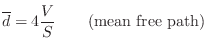
Mean Free Path
A rough guide to the average delay-line length is the ``mean free path'' in the desired reverberant environment. The mean free path is defined as the average distance a ray of sound travels before it encounters an obstacle and reflects. An approximate value for the mean free path, due to Sabine, an early pioneer of statistical room acoustics, is
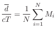
Mode Density Requirement
A guide for the sum of the delay-line lengths is the desired
mode density. The sum of delay-line lengths ![]() in a lossless
FDN is simply the order of the system
in a lossless
FDN is simply the order of the system ![]() :
:
Since the order of a system equals the number of poles, we have that
![]() is the number of poles on the unit circle in the lossless
prototype. If the modes were uniformly distributed, the mode density
would be
is the number of poles on the unit circle in the lossless
prototype. If the modes were uniformly distributed, the mode density
would be ![]() modes per Hz. Schroeder [417]
suggests that, for a reverberation time of 1 second, a mode density of
0.15 modes per Hz is adequate. Since the mode widths are inversely
proportional to reverberation time, the mode density for a
reverberation time of 2 seconds should be 0.3 modes per Hz, etc. In
summary, for a sufficient mode density in the frequency domain,
Schroeder's formula is
modes per Hz. Schroeder [417]
suggests that, for a reverberation time of 1 second, a mode density of
0.15 modes per Hz is adequate. Since the mode widths are inversely
proportional to reverberation time, the mode density for a
reverberation time of 2 seconds should be 0.3 modes per Hz, etc. In
summary, for a sufficient mode density in the frequency domain,
Schroeder's formula is
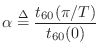
Prime Power Delay-Line Lengths
When the delay-line lengths need to be varied in real time, or
interactively in a GUI, it is convenient to choose each delay-line
length ![]() as an integer power of a distinct prime number
as an integer power of a distinct prime number ![]() [457]:
[457]:
Suppose we are initially given desired delay-line lengths ![]() arranged in ascending order so that
arranged in ascending order so that
![$\displaystyle \left[\frac{\log(M_i)}{\log(p_i)}\right]
\isdefs \left\lfloor 0.5 + \frac{\log(M_i)}{\log(p_i)}\right\rfloor.
$](http://www.dsprelated.com/josimages_new/pasp/img808.png)
This prime-power length scheme is used to keep 16 delay lines both variable and mutually prime in Faust's reverb_designer.dsp programming example (via the function prime_power_delays in effect.lib).
Achieving Desired Reverberation Times
A lossless prototype reverberator, as in Fig.3.10 when ![]() ,
has all of its poles on the unit circle in the
,
has all of its poles on the unit circle in the ![]() plane, and its
reverberation time is infinity. To set the reverberation time to a
desired value, we need to move the poles slightly inside the unit
circle. Furthermore, due to air absorption
(§2.3,§B.7.15), we want the high-frequency
poles to be more damped than the low-frequency poles
[314]. As discussed in §2.3, this type
of transformation can be obtained using the substitution
plane, and its
reverberation time is infinity. To set the reverberation time to a
desired value, we need to move the poles slightly inside the unit
circle. Furthermore, due to air absorption
(§2.3,§B.7.15), we want the high-frequency
poles to be more damped than the low-frequency poles
[314]. As discussed in §2.3, this type
of transformation can be obtained using the substitution
where
Solving for
The last form comes from
Series expanding
Conformal Map Interpretation of Damping Substitution
The relation
![]() [Eq.
[Eq.![]() (3.7)] can
be written down directly from
(3.7)] can
be written down directly from
![]() [Eq.
[Eq.![]() (3.5)] by interpreting Eq.
(3.5)] by interpreting Eq.![]() (3.5) as an approximate
conformal map [326] which takes each pole
(3.5) as an approximate
conformal map [326] which takes each pole
![]() ,
say, from the unit circle to the point
,
say, from the unit circle to the point
![]() .
Thus, the new pole radius is approximately
.
Thus, the new pole radius is approximately
![]() ,
where the approximation is valid when
,
where the approximation is valid when ![]() is approximately constant
between the new pole location and the unit circle. To see this,
consider the partial fraction expansion [449] of a proper
is approximately constant
between the new pole location and the unit circle. To see this,
consider the partial fraction expansion [449] of a proper
![]() th-order lossless transfer function
th-order lossless transfer function ![]() mapped to
mapped to
![]() :
:
![$\displaystyle H'(z)
= \sum_{k=1}^N \frac{r_k}{1-p_kG(z)z^{-1}}
= \sum_{k=1}^N r_k\left[1+p_kG(z)z^{-1}+p_k^2G^2(z)z^{-2}+\cdots\right],
$](http://www.dsprelated.com/josimages_new/pasp/img838.png)
Happily, while we may not know precisely where our poles have moved as
a result of introducing the per-sample damping filter ![]() , the
relation
, the
relation
![]() [Eq.
[Eq.![]() (3.6)] remains
exact at every frequency by construction, as it is based only on the
physical interpretation of each unit delay as a propagation delay for
a plane wave across one sampling interval
(3.6)] remains
exact at every frequency by construction, as it is based only on the
physical interpretation of each unit delay as a propagation delay for
a plane wave across one sampling interval ![]() , during which
(zero-phase) filtering by
, during which
(zero-phase) filtering by ![]() is assumed (§2.3). More
generally, we can design minimum-phase filters for which
is assumed (§2.3). More
generally, we can design minimum-phase filters for which
![]() , and neglect the resulting
phase dispersion.
, and neglect the resulting
phase dispersion.
In summary, we see that replacing ![]() by
by
![]() everywhere in the
FDN lossless prototype (or any lossless LTI system for that matter)
serves to move its poles away from the unit circle in the
everywhere in the
FDN lossless prototype (or any lossless LTI system for that matter)
serves to move its poles away from the unit circle in the ![]() plane
onto some contour inside the unit circle that provides the desired
decay time at each frequency.
plane
onto some contour inside the unit circle that provides the desired
decay time at each frequency.
A general design guideline for artificial reverberation applications
[217] is that all pole radii in the
reverberator should vary smoothly with frequency. This translates
to ![]() having a smooth frequency response. To see why this
is desired, consider momentarily the frequency-independent case in
which we desire the same reverberation time at all frequencies
(Fig.3.10 with real
having a smooth frequency response. To see why this
is desired, consider momentarily the frequency-independent case in
which we desire the same reverberation time at all frequencies
(Fig.3.10 with real ![]() , as drawn). In this case, it is
ideal for all of the poles to have this decay time. Otherwise, the
late decay of the impulse response will be dominated by the poles
having the largest magnitude, and it will be ``thinner'' than it was
at the beginning of the response when all poles were contributing to
the output. Only when all poles have the same magnitude will the late
response maintain the same modal density throughout the decay.
, as drawn). In this case, it is
ideal for all of the poles to have this decay time. Otherwise, the
late decay of the impulse response will be dominated by the poles
having the largest magnitude, and it will be ``thinner'' than it was
at the beginning of the response when all poles were contributing to
the output. Only when all poles have the same magnitude will the late
response maintain the same modal density throughout the decay.
Damping Filters for Reverberation Delay Lines
In an FDN, such as the one shown in Fig.3.10, delays ![]() appear
in long delay-line chains
appear
in long delay-line chains ![]() . Therefore, the filter needed at
the output (or input) of the
. Therefore, the filter needed at
the output (or input) of the ![]() th delay line is
th delay line is
![]() (replace
(replace
![]() by
by
![]() in Fig.3.10).4.15 However, because
in Fig.3.10).4.15 However, because
![]() is so close to
is so close to ![]() in magnitude, and because it varies so weakly
across the frequency axis, we can design a much lower-order filter
in magnitude, and because it varies so weakly
across the frequency axis, we can design a much lower-order filter
![]() that provides the desired attenuation
versus frequency to within psychoacoustic resolution. In fact,
perfectly nice reverberators can be designed in which
that provides the desired attenuation
versus frequency to within psychoacoustic resolution. In fact,
perfectly nice reverberators can be designed in which ![]() is
merely first order for each
is
merely first order for each ![]() [314,217].
[314,217].
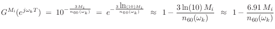
Delay-Line Damping Filter Design
Let
![]() denote the desired reverberation time at radian frequency
denote the desired reverberation time at radian frequency
![]() , and let
, and let ![]() denote the transfer function of the lowpass
filter to be placed in series with the
denote the transfer function of the lowpass
filter to be placed in series with the ![]() th delay line which is
th delay line which is ![]() samples long. The problem we consider now is how to design these
filters to yield the desired reverberation time. We will specify an
ideal amplitude response for
samples long. The problem we consider now is how to design these
filters to yield the desired reverberation time. We will specify an
ideal amplitude response for ![]() based on the desired
reverberation time at each frequency, and then use conventional
filter-design methods to obtain a low-order approximation to this
ideal specification.
based on the desired
reverberation time at each frequency, and then use conventional
filter-design methods to obtain a low-order approximation to this
ideal specification.
In accordance with Eq.![]() (3.6), the lowpass filter
(3.6), the lowpass filter ![]() in series
with a length
in series
with a length ![]() delay line should approximate
delay line should approximate
This is the same formula derived by Jot [217] using a somewhat different approach.
Now that we have specified the ideal delay-line filter
![]() in
terms of its amplitude response in dB, any number of filter-design
methods can be used to find a low-order
in
terms of its amplitude response in dB, any number of filter-design
methods can be used to find a low-order ![]() which provides a good
approximation to satisfying Eq.
which provides a good
approximation to satisfying Eq.![]() (3.9). Examples include the functions
invfreqz and stmcb in Matlab. Since the variation
in reverberation time is typically very smooth with respect to
(3.9). Examples include the functions
invfreqz and stmcb in Matlab. Since the variation
in reverberation time is typically very smooth with respect to
![]() , the filters
, the filters ![]() can be very low order.
can be very low order.
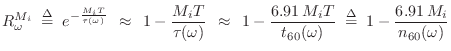
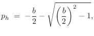
First-Order Delay-Filter Design
The first-order case is very simple while enabling separate control of
low-frequency and high-frequency reverberation times. For simplicity,
let's specify ![]() and
and
![]() , denoting the desired
decay-time at dc (
, denoting the desired
decay-time at dc (![]() ) and half the sampling rate
(
) and half the sampling rate
(
![]() ). Then we have determined the coefficients of a
one-pole filter:
). Then we have determined the coefficients of a
one-pole filter:
![\begin{eqnarray*}
\frac{g_i}{1-p_i} &=& 10^{-3 M_i T / t_{60}(0)}
\eqsp e^{-M_iT...
...(\pi/T)}
\eqsp e^{-M_iT/\tau(\pi/T)} \isdefs R_\pi^{M_i}\\ [5pt]
\end{eqnarray*}](http://www.dsprelated.com/josimages_new/pasp/img870.png)
where
![]() denotes the
denotes the ![]() th delay-line length in
seconds. These two equations are readily solved to yield
th delay-line length in
seconds. These two equations are readily solved to yield
![\begin{eqnarray*}
p_i &=& \frac{R_0^{M_i}-R_\pi^{M_i}}{R_0^{M_i}+R_\pi^{M_i}}\\ [5pt]
g_i &=& \frac{2R_0^{M_i}R_\pi^{M_i}}{R_0^{M_i}+R_\pi^{M_i}}
\end{eqnarray*}](http://www.dsprelated.com/josimages_new/pasp/img872.png)
The truncated series approximation
Orthogonalized First-Order Delay-Filter Design
In [217], first-order delay-line filters of the form

denotes the ratio of reverberation time at half the sampling rate divided by the reverberation time at dc.4.16
Multiband Delay-Filter Design
In §3.7.5, we derived first-order FDN delay-line filters which
can independently set the reverberation time at dc and at half the
sampling rate. However, perceptual studies indicate that
reverberation time should be independently adjustable in at least
three frequency bands [217]. To provide this degree
of control (and more), one can implement a multiband delay-line filter
using a general-purpose filter bank
[370,500]. The output, say, of each delay
line is split into ![]() bands, where
bands, where ![]() is recommended, and then,
from Eq.
is recommended, and then,
from Eq.![]() (3.6), the gain in the
(3.6), the gain in the ![]() th band for a length
th band for a length ![]() delay-line can be set to
delay-line can be set to
Spectral Coloration Equalizer
In the previous section, a ``graphical equalizer'' was used to set the
reverberator decay time independently in each spectral band slice.
While this gives much control over decay time, there is no control
over the initial spectral gain in each band. Therefore, another good
place for a graphical equalizer is at the reverberator input or
output. Such an equalizer allows control of the initial
spectral coloration of the reverberator. In the example of
Fig.3.10, a spectral coloration equalizer is most efficiently
applied to the input signal ![]() , before entering the FDN (but after
splitting off the direct signal to be scaled by
, before entering the FDN (but after
splitting off the direct signal to be scaled by ![]() and added to the
output), or the output of
and added to the
output), or the output of ![]() in Fig.3.10.
in Fig.3.10.
Tonal Correction Filter
Let ![]() denote the component of the impulse response arising from
the
denote the component of the impulse response arising from
the ![]() th pole of the system. Then the energy associated with that pole
is
th pole of the system. Then the energy associated with that pole
is
In the case of the first-order delay-line filters discussed in §3.7.5, good tonal correction is given by the following one-zero filter:

FDNs as Digital Waveguide Networks
As discussed in §C.15, the FDN using a
Householder-reflection feedback matrix
![]() is equivalent to a network of
is equivalent to a network of ![]() digital waveguides
intersecting at a single scattering junction
[463,464,385]. The wave impedance in the
digital waveguides
intersecting at a single scattering junction
[463,464,385]. The wave impedance in the ![]() th
waveguide is simply
th
waveguide is simply
![]() , the
, the ![]() th element of the
axis-of-reflection vector
th element of the
axis-of-reflection vector
![]() . The choice
. The choice
![]() corresponds to all of the waveguides having the same impedance (the
``isotrophic junction'' case).
corresponds to all of the waveguides having the same impedance (the
``isotrophic junction'' case).
FDN Reverberators in Faust
The Faust example reverb_designer.dsp brings up a
![]() FDN reverberator in which the signal out of each delay line is
split into five bands so that
FDN reverberator in which the signal out of each delay line is
split into five bands so that
![]() can be controlled
independently in each band. The 16 delay-line lengths are distributed
exponentially between a minimum and maximum length set by two
min/max-length sliders, but rounded to the nearest integer-power of a
distinct prime, as introduced above in §3.7.3). The FDN
reverberator is implemented in Faust's effect.lib. The
band-splitting is carried out by the filterbank function in
Faust's filter.lib.
can be controlled
independently in each band. The 16 delay-line lengths are distributed
exponentially between a minimum and maximum length set by two
min/max-length sliders, but rounded to the nearest integer-power of a
distinct prime, as introduced above in §3.7.3). The FDN
reverberator is implemented in Faust's effect.lib. The
band-splitting is carried out by the filterbank function in
Faust's filter.lib.
The Faust function filterbank(order,freqs) implements a filter bank having the needed properties using Butterworth lowpass/highpass band-splitting arranged in a dyadic tree (normally a good choice for audio filter banks). That is, the whole spectrum is split at the highest crossover frequency, the lowpass region is then split into two bands at the next crossover frequency down, and so on, splitting the lowpass band at each stage in the dyadic tree [455,500]. The number of poles in each Butterworth lowpass/highpass filter is specified by order, and freqs contains a list of desired crossover frequencies separating the bands. A certain amount of dispersion is also introduced, since the filter bank is causal and delay-equalized (so that the bands may be summed without phase cancellation artifacts at the band edges). Also note that the lower bands are effectively produced by higher order filters than the upper bands. When the reverberation time is longer than the dispersion delay, the dispersion should not be audible as such, although it can affect the ``sound'' of the reverberation. In general, however, artificial reverberators normally benefit from additional allpass dispersion.
Figure 3.12 shows the block diagram of a ![]() FDN
reverberator made from Faust's reverb_designer.dsp by
changing 16 to 4. Figure 3.13 shows the Faust block diagram of
the associated
FDN
reverberator made from Faust's reverb_designer.dsp by
changing 16 to 4. Figure 3.13 shows the Faust block diagram of
the associated ![]() Hamard matrix multiplication. As it shows,
multiplication by a Hadamard matrix can be implemented (ignoring the
normalizing scale factor) as a series of block sums and differences
(often called butterflies or shufflers) in which the
block size decreases by a factor of 2 each stage. Figures for the
remaining components of the reverberator may be perused via the shell
command faust2firefox reverb_designer.dsp followed by
clicking on the blocks in the browser.
Hamard matrix multiplication. As it shows,
multiplication by a Hadamard matrix can be implemented (ignoring the
normalizing scale factor) as a series of block sums and differences
(often called butterflies or shufflers) in which the
block size decreases by a factor of 2 each stage. Figures for the
remaining components of the reverberator may be perused via the shell
command faust2firefox reverb_designer.dsp followed by
clicking on the blocks in the browser.
![\includegraphics[width=\twidth]{eps/fdnrev0}](http://www.dsprelated.com/josimages_new/pasp/img894.png) |
![\includegraphics[width=\twidth]{eps/hadamard4}](http://www.dsprelated.com/josimages_new/pasp/img895.png)
Zita-Rev1
A FOSS4.17 reverberator that combines elements of Schroeder (§3.5) and FDN reverberators (§3.7) is zita-rev1,4.18written in C++ for Linux systems by Fons Adriaensen. A Faust version of the zita-rev1 stereo-mode functionality is zita_rev1 in Faust's effect.lib. A high-level block diagram appears in Fig.3.14.
![\includegraphics[width=\twidth]{eps/zita-rev1}](http://www.dsprelated.com/josimages_new/pasp/img897.png) |
The main high-level addition relative to an 8th-order FDN reverberator
is the block labeled allpass_combs in Fig.3.14.
This block inserts a Schroeder allpass comb filter (Fig.2.30) in
series with each delay line. In zita-rev1 (as of this
writing), the allpass-comb feedforward/feedback coefficients are all
set to ![]() . The delay-line lengths and other details are readily
found in the freely available source code (or by browsing the
Faust-generated block diagram).
. The delay-line lengths and other details are readily
found in the freely available source code (or by browsing the
Faust-generated block diagram).
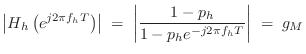
Zita-Rev1 Delay-Line Filters
In zita-rev1, the damping filter for each delay line consists
of a low-shelf filter ![]() [449],4.19in series with a unique first-order lowpass filter
[449],4.19in series with a unique first-order lowpass filter ![]() that sets
the high-frequency
that sets
the high-frequency ![]() to be half that of the middle-band at a
particular frequency
to be half that of the middle-band at a
particular frequency ![]() (specified as ``HF Damping'' in the GUI).
Since the filter
(specified as ``HF Damping'' in the GUI).
Since the filter ![]() is constrained to be a lowpass,
is constrained to be a lowpass,
![]() for
for ![]() , i.e., the decay time gets
shorter at higher frequencies.
, i.e., the decay time gets
shorter at higher frequencies.
Viewing the resulting damping filter
![]() as a
three-band filter bank (§3.7.5), let
as a
three-band filter bank (§3.7.5), let ![]() and
and ![]() denote the
desired band gains at dc and ``middle frequencies'',
respectively.4.20 Then the low shelf may be set for a
desired dc-gain of
denote the
desired band gains at dc and ``middle frequencies'',
respectively.4.20 Then the low shelf may be set for a
desired dc-gain of ![]() , and its input (or output) signal
multiplied by
, and its input (or output) signal
multiplied by ![]() to obtain the resulting filter
to obtain the resulting filter

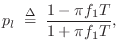
The lowpass filter ![]() is also first order, and to provide half
the middle-band
is also first order, and to provide half
the middle-band ![]() at the beginning of the ``high'' band, the
lowpass should ``break'' to a gain of
at the beginning of the ``high'' band, the
lowpass should ``break'' to a gain of ![]() at the ``HF Damping''
frequency
at the ``HF Damping''
frequency ![]() specified in the GUI. A unity-dc-gain one-pole
lowpass has the form [449]
specified in the GUI. A unity-dc-gain one-pole
lowpass has the form [449]

Further Extensions
Schroeder's original structures for artificial reverberation were comb filters and allpass filters made from two comb filters. Since then, they have been upgraded to include specific early reflections and per-sample air-absorption filtering (Moorer, Schroeder), precisely specified frequency dependent reverberation time (Jot), and a nearly independent factorization of ``coloration'' and ``duration'' aspects (Jot). The evolution from comb filters to feedback delay networks (Gerzon, Stautner, Puckette, Jot) can be seen as a means for obtaining greater richness of feedback, so that the diffuseness of the impulse response is greater than what is possible with parallel and/or series comb filters. In fact, an FDN can be seen as a richly cross-coupled bank of feedback comb filters whenever the diagonal of the feedback matrix is nonzero. The question then becomes what aspects of artificial reverberation have not yet been fully addressed?
Spatialization of Reverberant Reflections
While we did not go into the subject here, the early reflections should be spatialized by including a head-related transfer function (HRTF) on each tap of the early-reflection delay line [248].4.21
Some kind of spatialization may be needed also for the late reverberation. A true diffuse field (§3.2.1) consists of a sum of plane waves traveling in all directions in 3D space. Since we do not know how to achieve this effect using current systems for reverberation, the typical goal is to simply extract uncorrelated outputs from the reverberation network and feed them to the various output channels, as discussed in §3.5. However, this is not ideal, since the resulting sound field consists of wavefronts arriving from each of the speakers, and it is possible for the reverberation to sound like it is emanating from discrete speaker locations. It may be that spatialization of some kind can better fool the ear into believing the late reverberation is coming from all directions.
Distribution of Mode Frequencies
Another way in which current reverberation systems are ``artificial''
is the unnaturally uniform distribution of resonant modes with respect
to frequency. Because Schroeder, FDN, and waveguide reverbs are
all essentially a collection of ![]() delay lines with feedback around
them, the modes tend to be distributed as the superposition of the
resonant modes of
delay lines with feedback around
them, the modes tend to be distributed as the superposition of the
resonant modes of ![]() feedback comb filters. Since a feedback comb
filter has a nearly harmonic set of modes (see §2.6.2),
aggregates of comb filters tend to provide a uniform modal density in
the frequency domain. In real reverberant spaces, the mode density
increases as frequency squared, so it should be verified that the
uniform modes used in a reverberator are perceptually equivalent to
the increasingly dense modes in nature. Another aspect of perception
to consider is that frequency-domain perception of resonances actually
decreases with frequency. To summarize, in nature the modes get denser
with frequency, while in perception they are less resolved, and in
current reverberation systems they stay more or less uniform with
frequency; perhaps a uniform distribution is a good compromise between
nature and perception?
feedback comb filters. Since a feedback comb
filter has a nearly harmonic set of modes (see §2.6.2),
aggregates of comb filters tend to provide a uniform modal density in
the frequency domain. In real reverberant spaces, the mode density
increases as frequency squared, so it should be verified that the
uniform modes used in a reverberator are perceptually equivalent to
the increasingly dense modes in nature. Another aspect of perception
to consider is that frequency-domain perception of resonances actually
decreases with frequency. To summarize, in nature the modes get denser
with frequency, while in perception they are less resolved, and in
current reverberation systems they stay more or less uniform with
frequency; perhaps a uniform distribution is a good compromise between
nature and perception?
At low frequencies, however, resonant modes are accurately perceived in reverberation as boosts, resonances, and cuts. They are analogous to early reflections in the time domain, and we could call them the ``early resonances.'' It is interesting that no system for artificial reverberation except waveguide mesh reverberation (of which the author is aware) explicitly attempts precise shaping of the low-frequency amplitude response of a desired reverberant space, at least not directly. The low-frequency response is shaped indirectly by the choice of early reflections, and the use of parallel comb-filter banks in Schroeder reverberators serves also to shape the low-frequency response significantly. However, it would be possible to add filters for shaping more carefully the low-frequency response. Perhaps a reason for this omission is that hall designers work very hard to eliminate any explicit resonances or antiresonances in the response of a room. If uneven resonance at low frequencies is always considered a defect, then designing for a maximally uniform mode distribution, as has been discussed for the high-frequency modes, would be ideal also at low frequencies. Quite the opposite situation exists when designing ``small-box reverberators'' to simulate musical instrument resonators [428,203]; there, the low-frequency modes impart a characteristic timbre on the low-frequency resonance of the instrument (see Fig.3.2).
Digital Waveguide Reverberators
It was mentioned in §3.7.8 above that FDNs can be formulated as special cases of Digital Waveguide Networks (DWN) (see Appendix C for a fuller development of DWNs). Specifically, an FDN is obtained from a DWN consisting of a single scattering junction (§C.15). It follows that the DWN paradigm provides a more generalized framework in which to pursue further improvements of reverberation architecture. For example, when multiple FDNs are embedded within a single DWN, it becomes possible to richly cross-couple them in an energy-controlled manner in order to create richer recursive structures than either alone. General DWNs were proposed for artificial reverberation in [430,433].
The Digital Waveguide Mesh for Reverberation
A special case of digital waveguide networks known as the digital waveguide mesh has also been proposed for use in artificial reverberation systems [396,518].
As discussed in §2.4, a digital waveguide (bidirectional delay line) can be considered a computational acoustic model for traveling waves in opposite directions. A mesh of such waveguides in 2D or 3D can simulate waves traveling in any direction in the space. As an analogy, consider a tennis racket in which a rectilinear mesh of strings forms a pseudo-membrane.
A major advantage of the waveguide mesh for reverberation applications is that wavefronts are explicitly simulated in all directions, as in real reverberant spaces. Therefore, a true diffuse field can be developed in the late reverberation. Also, the echo density grows with time and the mode density grows with frequency in a natural manner for the 2D and 3D mesh. Finally, the low-frequency modes of the reverberant space can be simulated very precisely (for better or worse).
The computational cost of a waveguide mesh is made tractable relative to more conventional finite-difference simulations by (1) the use of multiply-free scattering junctions and (2) very coarse meshes. Use of a coarse mesh means that the ``physical modeling'' aspects of the mesh are only valid at low frequencies. As practical matter, this works out well because the ear cannot hear mode tuning errors at high frequencies. There is no error in the mode dampings in a lossless reverberator prototype, because the waveguide mesh is lossless by construction. Therefore, the only errors relative to an ideal simulation of a lossless membrane or space are (1) mode tuning error, and (2) finite band width (cut off at half the sampling rate). The tuning error can be understood as due to dispersion of the traveling waves in certain directions [518,399]. Much progress has been made on the problem of correcting this dispersion error in various mesh geometries (rectilinear, triangular, tetrahedral, etc.) [521,398,399].
See §C.14 for an introduction to the digital waveguide mesh and a few of its properties.
Time Varying Reverberators
In real rooms, thermal convention currents cause the propagation path delays to vary over time [58]. Therefore, for greater physical accuracy, the delay lines within a digital reverberator should vary over time. From a more practical perspective, time variation helps to break up and obscure unwanted repetition in the late reverberation impulse response [430,104].
Next Section:
Delay-Line and Signal Interpolation
Previous Section:
Acoustic Modeling with Digital Delay


