Sign in

Search Online Books

Free Online Books

Sponsor

Industry's highest performing at the lowest power DSPs now as low as $5.00*
Start development today!
*volume pricing for 10ku

Chapters

Physical Audio Signal Processing
    Virtual Musical Instruments
       Bowed Strings
          The Bow-String Scattering Junction

Chapter Contents:

Search Physical Audio Signal Processing

Book Index | Global Index

Would you like to be notified by email when Julius Orion Smith III publishes a new entry into his blog?

The Bow-String Scattering Junction

The theory of bow-string interaction is described in [95,151,244,307,308]. The basic operation of the bow is to reconcile the nonlinear bow-string friction curve with the string wave impedance :

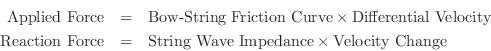
$\begin{eqnarray*} \mbox{Applied Force} &=& \mbox{Bow-String Friction Curve} \tim... ... &=& \mbox{String Wave Impedance} \times \mbox{Velocity Change} \end{eqnarray*}$

or, equating these equal and opposite forces, we obtain

$\displaystyle R_b(v_{\Delta})\times v_{\Delta}= R_s\left[v_{\Delta}^{+}- v_{\Delta}\right]$

where $v_{\Delta}=v_b-v_s$ is the velocity of the bow minus that of the string, $v_s=v_{sl}^{+}+v_{sl}^{-}=v_{sr}^{+}+v_{sr}^{-}$ is the string velocity in terms of traveling waves,

is the wave impedance of the string (equal to the geometric mean of tension and density), and $R_b(v_{\Delta})$ is the friction coefficient for the bow against the string, i.e., bow force $F_b(v_{\Delta}) = R_b(v_{\Delta}) \cdot v_{\Delta}$ . (Force and velocity point in the same direction when they have the same sign.) Here, $v_{sr}$ denotes transverse velocity on the segment of the bowed string to the right of the bow, and $v_{sl}$ denotes velocity waves to the left of the bow. The corresponding normalized functions to be used in the Friedlander-Keller graphical solution technique are depicted in Fig.9.53.

**Figure 9.53:** Overlay of normalized bow-string friction curve $R_b(v_{\Delta })/R_s$ with the string ``load line'' $v_{\Delta }^{+}- v_{\Delta }$ . The ``capture'' and ``break-away'' differential velocity is denoted $v_{\Delta }^c$ . Note that increasing the bow force increases $v_{\Delta }^c$ as well as enlarging the maximum force applied (at the peaks of the curve).
$\includegraphics[width=4in]{eps/fBowFrictionCurve}$

In a bowed string simulation as in Fig.9.51, a velocity input (which is injected equally in the left- and right-going directions) must be found such that the transverse force of the bow against the string is balanced by the reaction force of the moving string. If bow-hair dynamics are neglected [176], the bow-string interaction can be simulated using a memoryless table lookup or segmented polynomial in a manner similar to single-reed woodwinds [431].

A derivation analogous to that for the single reed is possible for the simulation of the bow-string interaction. The final result is as follows.

$\displaystyle v_{sr}^{-}$	$\displaystyle =$	$\displaystyle v_{sl}^{+}+ \hat\rho (v_{\Delta}^{+})\cdot v_{\Delta}^{+}$
$\displaystyle v_{sl}^{-}$	$\displaystyle =$	$\displaystyle v_{sr}^{+}+ \hat\rho (v_{\Delta}^{+})\cdot v_{\Delta}^{+}$

where $v_{\Delta}^{+}\isdef v_b-(v_{sr}^{+}+v_{sl}^{+})$ ,

is bow velocity, and

$\displaystyle \hat\rho (v_{\Delta}^{+})=\frac{r(v_{\Delta}(v_{\Delta}^{+}))}{1 + r(v_{\Delta}(v_{\Delta}^{+}))}$

The impedance ratio is defined as $r(v_{\Delta})=0.25R_b(v_{\Delta})/R_s$ ,

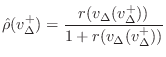
Nominally, $R_b(v_{\Delta})$ is constant (the so-called static coefficient of friction) for $\vert v_{\Delta}\vert\leq v_{\Delta}^c$ , where $v_{\Delta }^c$ is both the capture and break-away differential velocity. For $\vert v_{\Delta}\vert>v_{\Delta}^c$ , $R_b(v_{\Delta})$ falls quickly to a low dynamic coefficient of friction. It is customary in the bowed-string physics literature to assume that the dynamic coefficient of friction continues to approach zero with increasing $\vert v_{\Delta}\vert>v_{\Delta}^c$ [308,95].

**Figure 9.54:** Simple, qualitatively chosen bow table for the digital waveguide violin.
$\includegraphics[width=4in]{eps/fBowTable}$

Figure 9.54 illustrates a simplified, piecewise linear bow table $\hat\rho (v_{\Delta}^{+})$ . The flat center portion corresponds to a fixed reflection coefficient ``seen'' by a traveling wave encountering the bow stuck against the string, and the outer sections of the curve give a smaller reflection coefficient corresponding to the reduced bow-string interaction force while the string is slipping under the bow. The notation $v_{\Delta }^c$ at the corner point denotes the capture or break-away differential velocity. Note that hysteresis is neglected.

Previous: Digital Waveguide Bowed-String
Next: Bowed String Synthesis Extensions

Order a Hardcopy of Physical Audio Signal Processing

About the Author: Julius Orion Smith III
Julius Smith's background is in electrical engineering (BS Rice 1975, PhD Stanford 1983). He is presently Professor of Music and Associate Professor (by courtesy) of Electrical Engineering at Stanford's Center for Computer Research in Music and Acoustics (CCRMA), teaching courses and pursuing research related to signal processing applied to music and audio systems. See http://ccrma.stanford.edu/~jos/ for details.

Comments

No comments yet for this page

Add a Comment

You need to login before you can post a comment (best way to prevent spam). ( Not a member? )