


Digital Waveguide Filters
A Digital Waveguide Filter (DWF) can be defined as any digital filter built by stringing together digital waveguides.C.7 In the case of a cascade combination of unit-length waveguide sections, they are essentially the same as microwave filters [372] and unit element filters [136] (Appendix F). This section shows how DWFs constructed as a cascade chain of waveguide sections, and reflectively terminated, can be transformed via elementary manipulations to well known ladder and lattice digital filters, such as those used in speech modeling [297,363].
DWFs may be derived conceptually by sampling the unidirectional traveling waves in a system of ideal, lossless waveguides. Sampling is across time and space. Thus, variables in a DWF structure are equal exactly (at the sampling times and positions, to within numerical precision) to variables propagating in the physical medium in an interconnection of uniform 1D waveguides.
Ladder Waveguide Filters
An important class of DWFs can be constructed as a linear cascade
chain of digital waveguide sections, as shown in Fig.C.24 (a
slightly abstracted version of Fig.C.19). Each block labeled
![]() stands for a state-less Kelly-Lochbaum scattering junction
(§C.8.4) interfacing between wave impedances
stands for a state-less Kelly-Lochbaum scattering junction
(§C.8.4) interfacing between wave impedances ![]() and
and ![]() . We call this a ladder waveguide filter structure.
It is an exact bandlimited discrete-time model of a sequence of wave
impedances
. We call this a ladder waveguide filter structure.
It is an exact bandlimited discrete-time model of a sequence of wave
impedances ![]() , as used in the Kelly-Lochbaum piecewise-cylindrical
acoustic-tube model for the vocal tract in the context of voice
synthesis (Fig.6.2). The delays between scattering
junctions along both the top and bottom signal paths make it possible
to compute all of the scattering junctions in parallel--a property
that is becoming increasingly valuable in signal-processing
architectures.
, as used in the Kelly-Lochbaum piecewise-cylindrical
acoustic-tube model for the vocal tract in the context of voice
synthesis (Fig.6.2). The delays between scattering
junctions along both the top and bottom signal paths make it possible
to compute all of the scattering junctions in parallel--a property
that is becoming increasingly valuable in signal-processing
architectures.
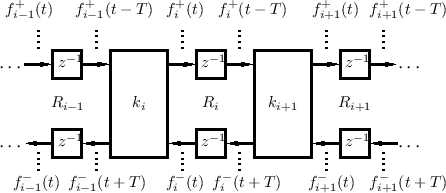
To transform the DWF of Fig.C.24 to a conventional ladder digital filter structure, as used in speech modeling [297,363], we need to (1) terminate on the right with a pure reflection and (2) eliminate the delays along the top signal path. We will do this in stages so as to point out a valuable intermediate case.
Reflectively Terminated Waveguide Filters
A reflecting termination occurs when the wave impedance of the next section is either zero or infinity (§C.8.1). Since Fig.C.24 is labeled for force waves, an infinite terminating impedance on the right results in
Half-Rate Ladder Waveguide Filters
The delays preceding the two inputs to each scattering junction can be ``pushed'' into the junction and then ``pulled'' out to the outputs and combine with the delays there. (This is easy to show using the Kelly-Lochbaum scattering junction derived in §C.8.4.) By performing this operation on every other section in the DWF chain, the half-rate ladder waveguide filter shown in Fig.C.25 is obtained [432].
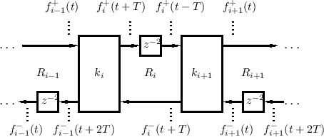
This ``half-rate'' ladder DWF is so-called because its sampling rate can be cut in half due to each delay being two-samples long. It has advantages worth considering, which will become clear after we have derived conventional ladder digital filters below. Note that now pairs of scattering junctions can be computed in parallel, and an exact physical interpretation remains. That is, it can still be used as a general purpose physical modeling building block in this more efficient (half-rate) form.
Note that when the sampling rate is halved, the physical wave
variables (computed by summing two traveling-wave components) are at
the same time only every other spatial sample. In particular, the
physical transverse forces on the right side of scattering junctions
![]() and
and ![]() in Fig.C.25 are
in Fig.C.25 are
![\begin{eqnarray*}
f_i(t+T)&=&f^{{+}}_i(t+T)+f^{{-}}_i(t+T)\\ [5pt]
f_{i+1}(t)&=&f^{{+}}_{i+1}(t)+f^{{-}}_{i+1}(t) \end{eqnarray*}](http://www.dsprelated.com/josimages_new/pasp/img3681.png)
respectively. In the half-rate case, adjacent spatial samples are
separated in time by half a temporal sample ![]() . If physical
variables are needed only for even-numbered (or odd-numbered) spatial
samples, then there is no relative time skew, but more generally,
things like collision detection, such as for slap-bass string-models
(§9.1.6), can be affected. In summary, the half-rate ladder
waveguide filter has an alternating half-sample time skew from section
to section when used as a physical modeling building block.
. If physical
variables are needed only for even-numbered (or odd-numbered) spatial
samples, then there is no relative time skew, but more generally,
things like collision detection, such as for slap-bass string-models
(§9.1.6), can be affected. In summary, the half-rate ladder
waveguide filter has an alternating half-sample time skew from section
to section when used as a physical modeling building block.
Conventional Ladder Filters
Given a reflecting termination on the right, the half-rate DWF chain of Fig.C.25 can be reduced further to the conventional ladder/lattice filter structure shown in Fig.C.26.
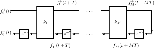
To make a standard ladder/lattice filter, the sampling rate is cut in
half (i.e., replace ![]() by
by ![]() ), and the scattering junctions are
typically implemented in one-multiply form (§C.8.5) or
normalized form (§C.8.6), etc. Conventionally, if the
graph of the scattering junction is nonplanar, as it is for the
one-multiply junction, the filter is called a lattice filter;
it is called a ladder filter when the graph is planar, as it is
for normalized and Kelly-Lochbaum scattering junctions. For all-pole
transfer functions
), and the scattering junctions are
typically implemented in one-multiply form (§C.8.5) or
normalized form (§C.8.6), etc. Conventionally, if the
graph of the scattering junction is nonplanar, as it is for the
one-multiply junction, the filter is called a lattice filter;
it is called a ladder filter when the graph is planar, as it is
for normalized and Kelly-Lochbaum scattering junctions. For all-pole
transfer functions
![]() , the Durbin
recursion can be used to compute the reflection coefficients
, the Durbin
recursion can be used to compute the reflection coefficients ![]() from the desired transfer-function denominator polynomial coefficients
[449]. To implement arbitrary transfer-function zeros, a
linear combination of delay-element outputs is formed using weights
that are called ``tap parameters'' [173,297].
from the desired transfer-function denominator polynomial coefficients
[449]. To implement arbitrary transfer-function zeros, a
linear combination of delay-element outputs is formed using weights
that are called ``tap parameters'' [173,297].
To create Fig.C.26 from Fig.C.24, all delays along the top rail
are pushed to the right until they have all been worked around to the
bottom rail. In the end, each bottom-rail delay becomes ![]() seconds
instead of
seconds
instead of ![]() seconds. Such an operation is possible because of the
termination at the right by an infinite (or zero) wave impedance.
Note that there is a progressive one-sample time advance from section
to section. The time skews for the right-going (or left-going)
traveling waves can be determined simply by considering how many
missing (or extra) delays there are between that signal and the
unshifted signals at the far left.
seconds. Such an operation is possible because of the
termination at the right by an infinite (or zero) wave impedance.
Note that there is a progressive one-sample time advance from section
to section. The time skews for the right-going (or left-going)
traveling waves can be determined simply by considering how many
missing (or extra) delays there are between that signal and the
unshifted signals at the far left.
Due to the reflecting termination, conventional lattice filters cannot
be extended to the right in any physically meaningful way. Also,
creating network topologies more complex than a simple linear cascade
(or acyclic tree) of waveguide sections is not immediately possible
because of the delay-free path along the top rail. In particular, the
output ![]() cannot be fed back to the input
cannot be fed back to the input ![]() . Nevertheless,
as we have derived, there is an exact physical interpretation (with
time skew) for the conventional ladder/lattice digital filter.
. Nevertheless,
as we have derived, there is an exact physical interpretation (with
time skew) for the conventional ladder/lattice digital filter.
Power-Normalized Waveguide Filters
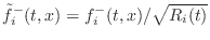
Above, we adopted the convention that the time variation of the wave
impedance did not alter the traveling force waves ![]() . In this
case, the power represented by a traveling force wave is modulated by
the changing wave impedance as it propagates. The signal power
becomes inversely proportional to wave impedance:
. In this
case, the power represented by a traveling force wave is modulated by
the changing wave impedance as it propagates. The signal power
becomes inversely proportional to wave impedance:
![$\displaystyle {\cal I}_i(t,x)
= {\cal I}^{+}_i(t,x)+{\cal I}^{-}_i(t,x)
= \frac{[f^{{+}}_i(t,x)]^2-[f^{{-}}_i(t,x)]^2}{R_i(t)}
$](http://www.dsprelated.com/josimages_new/pasp/img3691.png)
In [432,433], three methods are discussed for making signal power invariant with respect to time-varying branch impedances:
- The normalized waveguide scheme compensates for power
modulation by scaling the signals leaving the delays so as to give
them the same power coming out as they had going in. It requires two
additional scaling multipliers per waveguide junction.
- The normalized wave approach [297] propagates
rms-normalized waves in the waveguide. In this case, each
delay-line contains
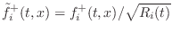 and
and
 . In this case, the power
stored in the delays does not change when the wave impedance
changes. This is the basis of the normalized ladder filter
(NLF) [174,297]. Unfortunately, four
multiplications are obtained at each scattering junction.
. In this case, the power
stored in the delays does not change when the wave impedance
changes. This is the basis of the normalized ladder filter
(NLF) [174,297]. Unfortunately, four
multiplications are obtained at each scattering junction.
- The transformer-normalized waveguide approach changes the
wave impedance at the output of the delay back to what it was at the
time it entered the delay using a ``transformer'' (defined in
§C.16).
The transformer-normalized DWF junction is shown in Fig.C.27
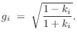
[432]. As derived in §C.16, the transformer ``turns
ratio'' ![]() is given by
is given by
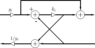 |
So, as in the normalized waveguide case, for the price of two extra multiplies per section, we can implement time-varying digital filters which do not modulate stored signal energy. Moreover, transformers enable the scattering junctions to be varied independently, without having to propagate time-varying impedance ratios throughout the waveguide network.
It can be shown [433] that cascade waveguide chains built using transformer-normalized waveguides are equivalent to those using normalized-wave junctions. Thus, the transformer-normalized DWF in Fig.C.27 and the wave-normalized DWF in Fig.C.22 are equivalent. One simple proof is to start with a transformer (§C.16) and a Kelly-Lochbaum junction (§C.8.4), move the transformer scale factors inside the junction, combine terms, and arrive at Fig.C.22. One practical benefit of this equivalence is that the normalized ladder filter (NLF) can be implemented using only three multiplies and three additions instead of the usual four multiplies and two additions.
The transformer-normalized scattering junction is also the basis of the digital waveguide oscillator (§C.17).
Next Section:
``Traveling Waves'' in Lumped Systems
Previous Section:
Scattering at Impedance Changes


