


Digital Waveguide Mesh
In §C.12, the theory of multiport scattering was derived, i.e.,
the reflections and transmissions that occur when ![]() digital
waveguides having wave impedances
digital
waveguides having wave impedances ![]() are connected together. It
was noted that when
are connected together. It
was noted that when ![]() is a power of two, there are
no multiplies in the scattering relations Eq.
is a power of two, there are
no multiplies in the scattering relations Eq.![]() (C.105), and that
this fact has been used to build multiply-free reverberators and other
structures using digital waveguide meshes
[430,518,146,396,520,521,398,399,401,55,202,321,320,322,422,33].
(C.105), and that
this fact has been used to build multiply-free reverberators and other
structures using digital waveguide meshes
[430,518,146,396,520,521,398,399,401,55,202,321,320,322,422,33].
The Rectilinear 2D Mesh
![\includegraphics[width=4in]{eps/SchematicWaveguideMesh}](http://www.dsprelated.com/josimages_new/pasp/img4008.png)
Figure C.32 shows the basic layout of the rectilinear 2D waveguide mesh. It can be thought of as simulating a plane using 1D digital waveguides in the same way that a tennis racket acts as a membrane composed of 1D strings.
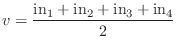
At each node (string intersection), we have the following simple formula for the
node velocity ![]() in terms of the four incoming traveling-wave components:
in terms of the four incoming traveling-wave components:
Dispersion
Since the digital waveguide mesh is lossless by construction (when modeling lossless membranes and volumes), and since it is also linear and time-invariant by construction, being made of ordinary digital filtering computations, there is only one type of error exhibited by the mesh: dispersion. Dispersion can be quantified as an error in propagation speed as a function of frequency and direction along the mesh. The mesh geometry (rectilinear, triangular, hexagonal, tetrahedral, etc.) strongly influences the dispersion properties. Many cases are analyzed in [55] using von Neumann analysis (see also Appendix D).
The triangular waveguide mesh [146] turns out to be the simplest mesh geometry in 2D having the least dispersion variation as a function of direction of propagation on the mesh. In other terms, the triangular mesh is closer to isotropic than all other known elementary geometries. The interpolated waveguide mesh [398] can also be configured to optimize isotropy, but at a somewhat higher compuational cost.
Recent Developments
An interesting approach to dispersion compensation is based on frequency-warping the signals going into the mesh [399]. Frequency warping can be used to compensate frequency-dependent dispersion, but it does not address angle-dependent dispersion. Therefore, frequency-warping is used in conjunction with an isotropic mesh.
The 3D waveguide mesh [518,521,399] is seeing more use for efficient simulation of acoustic spaces [396,182]. It has also been applied to statistical modeling of violin body resonators in [203,202,422,428], in which the digital waveguide mesh was used to efficiently model only the ``reverberant'' aspects of a violin body's impulse response in statistically matched fashion (but close to perceptually equivalent). The ``instantaneous'' filtering by the violin body is therefore modeled using a separate equalizer capturing the important low-frequency body and air modes explicitly. A unified view of the digital waveguide mesh and wave digital filters (§F.1) as particular classes of energy invariant finite difference schemes (Appendix D) appears in [54]. The problem of modeling diffusion at a mesh boundary was addressed in [268], and maximally diffusing boundaries, using quadratic residue sequences, was investigated in [279]; an introduction to this topic is given in §C.14.6 below.
2D Mesh and the Wave Equation
 |
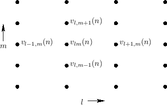
Consider the 2D rectilinear mesh, with nodes at positions ![]() and
and
![]() , where
, where ![]() and
and ![]() are integers, and
are integers, and ![]() and
and ![]() denote the
spatial sampling intervals along
denote the
spatial sampling intervals along ![]() and
and ![]() , respectively
(see Fig.C.33).
Then from
Eq.
, respectively
(see Fig.C.33).
Then from
Eq.![]() (C.105) the junction velocity
(C.105) the junction velocity ![]() at time
at time ![]() is given
by
is given
by
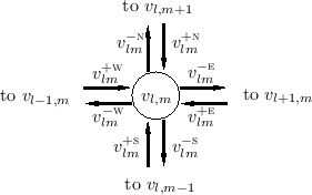
These incoming traveling-wave components arrive from the four
neighboring nodes after a one-sample propagation delay. For example,
![]() , arriving from the north, departed from node
, arriving from the north, departed from node
![]() at time
at time ![]() , as
, as
![]() .
Furthermore, the outgoing components at time
.
Furthermore, the outgoing components at time
![]() will arrive at the neighboring nodes
one sample in the future at time
will arrive at the neighboring nodes
one sample in the future at time ![]() .
For example,
.
For example,
![]() will become
will become
![]() .
Using these relations, we can
write
.
Using these relations, we can
write
![]() in terms of the four outgoing waves from its
neighbors at time
in terms of the four outgoing waves from its
neighbors at time ![]() :
:
where, for instance,
This may be shown in detail by writing
![\begin{eqnarray*}
v_{lm}(n-1)
&=& \frac{1}{2}[v_{lm}^{+\textsc{n}}(n-1) + \cdot...
...}^{-\textsc{n}}(n-1) + \cdots + v_{lm}^{-\textsc{w}}(n-1)\right]
\end{eqnarray*}](http://www.dsprelated.com/josimages_new/pasp/img4027.png)
so that
![\begin{eqnarray*}
v_{lm}(n-1)
&=& \frac{1}{2}[v_{lm}^{-\textsc{n}}(n-1) + \cdot...
...
v_{l,m-1}^{+\textsc{n}}(n) +
v_{l-1,m}^{+\textsc{e}}(n)\right].
\end{eqnarray*}](http://www.dsprelated.com/josimages_new/pasp/img4028.png)
Adding Equations (C.116-C.116), replacing
terms such as
![]() with
with
![]() , yields a computation in terms of physical node velocities:
, yields a computation in terms of physical node velocities:
![\begin{eqnarray*}
\lefteqn{v_{lm}(n+1) + v_{lm}(n-1) = } \\
& & \frac{1}{2}\left[
v_{l,m+1}(n) +
v_{l+1,m}(n) +
v_{l,m-1}(n) +
v_{l-1,m}(n)\right]
\end{eqnarray*}](http://www.dsprelated.com/josimages_new/pasp/img4031.png)
Thus, the rectangular waveguide mesh satisfies this equation
giving a formula for the velocity at node ![]() , in terms of
the velocity at its neighboring nodes one sample earlier, and itself
two samples earlier. Subtracting
, in terms of
the velocity at its neighboring nodes one sample earlier, and itself
two samples earlier. Subtracting
![]() from both sides yields
from both sides yields
![\begin{eqnarray*}
\lefteqn{v_{lm}(n+1) - 2 v_{lm}(n) + v_{lm}(n-1)} \\
&=& \fra...
.... \left[v_{l+1,m}(n) - 2 v_{lm}(n) + v_{l-1,m}(n)\right]\right\}
\end{eqnarray*}](http://www.dsprelated.com/josimages_new/pasp/img4033.png)
Dividing by the respective sampling intervals, and assuming ![]() (square mesh-holes), we obtain
(square mesh-holes), we obtain
![\begin{eqnarray*}
\lefteqn{\frac{v_{lm}(n+1) - 2 v_{lm}(n) + v_{lm}(n-1)}{T^2}} ...
...ft.\frac{v_{l+1,m}(n) - 2 v_{lm}(n) + v_{l-1,m}(n)}{X^2}\right].
\end{eqnarray*}](http://www.dsprelated.com/josimages_new/pasp/img4035.png)
In the limit, as the sampling intervals ![]() approach zero such that
approach zero such that
![]() remains
constant, we recognize these expressions as the definitions of the partial
derivatives with respect to
remains
constant, we recognize these expressions as the definitions of the partial
derivatives with respect to ![]() ,
, ![]() , and
, and ![]() , respectively, yielding
, respectively, yielding
![$\displaystyle \frac{\partial^2 v(t,x,y)}{\partial t^2} = \frac{X^2}{2T^2}
\left...
...^2 v(t,x,y)}{\partial x^2}
+ \frac{\partial^2 v(t,x,y)}{\partial y^2}
\right].
$](http://www.dsprelated.com/josimages_new/pasp/img4038.png)
![$\displaystyle \frac{\partial^2 v}{\partial t^2} =
c^2
\left[
\frac{\partial^2 v}{\partial x^2}
+ \frac{\partial^2 v}{\partial y^2}
\right]
$](http://www.dsprelated.com/josimages_new/pasp/img4040.png)
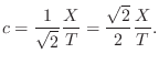
Discussion regarding solving the 2D wave equation subject to boundary conditions appears in §B.8.3. Interpreting this value for the wave propagation speed
The Lossy 2D Mesh
Because the finite-difference form of the digital waveguide mesh is the more efficient computationally than explicitly computing scattering wave variables (too see this, count the multiplies required per node), it is of interest to consider the finite-difference form also in the case of frequency-dependent losses. The method of §C.5.5 extends also to the waveguide mesh, which can be shown by generalizing the results of §C.14.4 above using the technique of §C.5.5.
The basic idea is once again that wave propagation during one sampling
interval (in time) is associated with linear filtering by ![]() .
That is,
.
That is, ![]() is regarded as the per-sample wave propagation filter.
is regarded as the per-sample wave propagation filter.
Diffuse Reflections in the Waveguide Mesh
In [416], Manfred Schroeder proposed the design of a
diffuse reflector based on a quadratic residue sequence. A
quadratic residue sequence ![]() corresponding to a prime number
corresponding to a prime number
![]() is the sequence
is the sequence ![]() mod
mod ![]() , for all integers
, for all integers ![]() . The sequence
is periodic with period
. The sequence
is periodic with period ![]() , so it is determined by
, so it is determined by ![]() for
for
![]() (i.e., one period of the infinite sequence).
(i.e., one period of the infinite sequence).
For example, when ![]() , the first period of the quadratic residue
sequence is given by
, the first period of the quadratic residue
sequence is given by
![\begin{eqnarray*}
a_7 &=& [0^2,1^2,2^2,3^2,4^2,5^2,6^2] \quad (\mbox{mod }7)\\
&=& [0, 1, 4, 2, 2, 4, 1]
\end{eqnarray*}](http://www.dsprelated.com/josimages_new/pasp/img4047.png)
An amazing property of these sequences is that their Fourier transforms have precisely constant magnitudes. That is, the sequence
![$\displaystyle \vert C_p(\omega_k)\vert \isdef \vert\dft _k(c_p)\vert
\isdef \l...
...^{p-1} c_p(n) e^{-j2\pi nk/p}\right\vert
= \sqrt{p}, \quad \forall k\in[0,p-1]
$](http://www.dsprelated.com/josimages_new/pasp/img4049.png)
Figure C.35 presents a simple matlab script which demonstrates the constant-magnitude Fourier property for all odd integers from 1 to 99.
function [c] = qrsfp(Ns)
%QRSFP Quadratic Residue Sequence Fourier Property demo
  if (nargin<1)
     Ns = 1:2:99; % Test all odd integers from 1 to 99
  end
  for N=Ns
    a = mod([0:N-1].^2,N);
    c = zeros(N-1,N);
    CM = zeros(N-1,N);
    c = exp(j*2*pi*a/N);
    CM = abs(fft(c))*sqrt(1/N);
    if (abs(max(CM)-1)>1E-10) || (abs(min(CM)-1)>1E-10)
       warn(sprintf("Failure for N=%d",N));
    end
  end
  r = exp(2i*pi*[0:100]/100); % a circle
  plot(real(r), imag(r),"k"); hold on;
  plot(c,"-*k"); % plot sequence in complex plane
end
|
Quadratic residue diffusers have been applied as boundaries of a 2D digital waveguide mesh in [279]. An article reviewing the history of room acoustic diffusers may be found in [94].
Next Section:
FDNs as Digital Waveguide Networks
Previous Section:
Two Coupled Strings


