


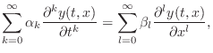
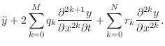
Digital Waveguide Theory
In this appendix, the basic principles of digital waveguide acoustic modeling are derived from a mathematical point of view. For this, the reader is expected to have some background in linear systems and elementary physics. In particular, facility with Laplace transforms [284], Newtonian mechanics [180], and basic differential equations is assumed.
We begin with the partial differential equation (PDE) describing the ideal vibrating string, which we first digitize by converting partial derivatives to finite differences. This yields a discrete-time recursion which approximately simulates the ideal string. Next, we go back and solve the original PDE, obtaining continuous traveling waves as the solution. These traveling waves are then digitized by ordinary sampling, resulting in the digital waveguide model for the ideal string. The digital waveguide simulation is then shown to be equivalent to a particular finite-difference recursion. (This only happens for the lossless ideal vibrating string with a particular choice of sampling intervals, so it is an interesting case.) Next digital waveguides simulating lossy and dispersive vibrating strings are derived, and alternative choices of wave variables (displacement, velocity, slope, force, power, etc.) are derived. Finally, an introduction to scattering theory for digital waveguides is presented.
The Ideal Vibrating String
![\includegraphics[width=\twidth]{eps/Fphysicalstring}](http://www.dsprelated.com/josimages_new/pasp/img3204.png)
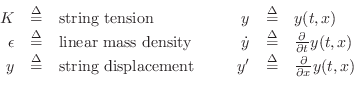
The wave equation for the ideal (lossless, linear, flexible) vibrating string, depicted in Fig.C.1, is given by
where
 |
where ``
The Finite Difference Approximation
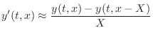
In the musical acoustics literature, the normal method for creating a computational model from a differential equation is to apply the so-called finite difference approximation (FDA) in which differentiation is replaced by a finite difference (see Appendix D) [481,311]. For example
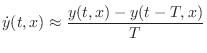
and
where
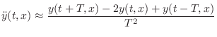

The odd-order derivative approximations suffer a half-sample delay error while all even order cases can be compensated as above.
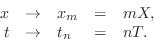
FDA of the Ideal String
Substituting the FDA into the wave equation gives

![$\displaystyle \frac{KT^2}{\epsilon X^2}
\left[ y(t,x+X) - 2 y(t,x) + y(t,x-X)\right]$](http://www.dsprelated.com/josimages_new/pasp/img3213.png)
In a practical implementation, it is common to set
Thus, to update the sampled string displacement, past values are needed for each point along the string at time instants
Perhaps surprisingly, it is shown in Appendix E that the above recursion is exact at the sample points in spite of the apparent crudeness of the finite difference approximation [442]. The FDA approach to numerical simulation was used by Pierre Ruiz in his work on vibrating strings [392], and it is still in use today [74,75].
When more terms are added to the wave equation, corresponding to complex
losses and dispersion characteristics, more terms of the form
![]() appear in (C.6). These higher-order terms correspond to
frequency-dependent losses and/or dispersion characteristics in
the FDA. All linear differential equations with constant coefficients give rise to
some linear, time-invariant discrete-time system via the FDA.
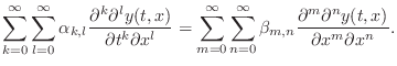
A general subclass of the linear, time-invariant case
giving rise to ``filtered waveguides'' is
appear in (C.6). These higher-order terms correspond to
frequency-dependent losses and/or dispersion characteristics in
the FDA. All linear differential equations with constant coefficients give rise to
some linear, time-invariant discrete-time system via the FDA.
A general subclass of the linear, time-invariant case
giving rise to ``filtered waveguides'' is
 |
(C.7) |
while the fully general linear, time-invariant 2D case is
 |
(C.8) |
A nonlinear example is
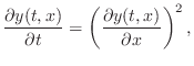 |
(C.9) |
and a time-varying example can be given by
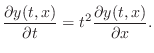 |
(C.10) |
Traveling-Wave Solution
It is easily shown that the lossless 1D wave equation
![]() is solved by any string shape which travels to the left or right with
speed
is solved by any string shape which travels to the left or right with
speed
![]() . Denote right-going
traveling waves in general by
. Denote right-going
traveling waves in general by
![]() and left-going
traveling waves by
and left-going
traveling waves by
![]() , where
, where ![]() and
and ![]() are assumed
twice-differentiable.C.1Then a general class of solutions to the
lossless, one-dimensional, second-order wave equation can be expressed
as
are assumed
twice-differentiable.C.1Then a general class of solutions to the
lossless, one-dimensional, second-order wave equation can be expressed
as
The next section derives the result that
An important point to note about the traveling-wave solution of the 1D
wave equation is that a function of two variables ![]() has been
replaced by two functions of a single variable in time units. This
leads to great reductions in computational complexity.
has been
replaced by two functions of a single variable in time units. This
leads to great reductions in computational complexity.
The traveling-wave solution of the wave equation was first published by d'Alembert in 1747 [100]. See Appendix A for more on the history of the wave equation and related topics.
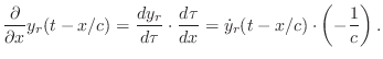
Traveling-Wave Partial Derivatives
Because we have defined our traveling-wave components
![]() and
and
![]() as having arguments in units of time, the partial
derivatives with respect to time
as having arguments in units of time, the partial
derivatives with respect to time ![]() are identical to simple
derivatives of these functions. Let
are identical to simple
derivatives of these functions. Let
![]() and
and
![]() denote the
(partial) derivatives with respect to time of
denote the
(partial) derivatives with respect to time of ![]() and
and ![]() ,
respectively. In contrast, the partial derivatives with respect to
,
respectively. In contrast, the partial derivatives with respect to ![]() are
are
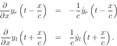
Denoting the spatial
partial derivatives by ![]() and
and
![]() , respectively, we can write more succinctly
, respectively, we can write more succinctly
![\begin{eqnarray*}
y'_r&=& -\frac{1}{c}{\dot y}_r\\ [5pt]
y'_l&=& \frac{1}{c}{\dot y}_l,
\end{eqnarray*}](http://www.dsprelated.com/josimages_new/pasp/img3234.png)
where this argument-free notation assumes the same ![]() and
and ![]() for all
terms in each equation, and the subscript
for all
terms in each equation, and the subscript ![]() or
or ![]() determines
whether the omitted argument is
determines
whether the omitted argument is ![]() or
or ![]() .
.
Now we can see that the second partial derivatives in ![]() are
are

These relations, together with the fact that partial differention is a linear operator, establish that
Use of the Chain Rule
These traveling-wave partial-derivative relations may be derived a bit
more formally by means of the chain rule from calculus, which
states that, for the composition of functions ![]() and
and ![]() , i.e.,
, i.e.,
To apply the chain rule to the spatial differentiation of traveling waves, define
![\begin{eqnarray*}
g_r(t,x) &=& t - \frac{x}{c}\\ [10pt]
g_l(t,x) &=& t + \frac{x}{c}.
\end{eqnarray*}](http://www.dsprelated.com/josimages_new/pasp/img3242.png)
Then the traveling-wave components can be written as
![]() and
and
![]() , and their partial derivatives with respect to
, and their partial derivatives with respect to ![]() become
become
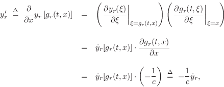
and similarly for ![]() .
.
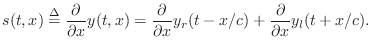
String Slope from Velocity Waves
Let's use the above result to derive the slope of the ideal
vibrating string
From Eq.![]() (C.11), we have the string displacement given by
(C.11), we have the string displacement given by
Wave Velocity
Because ![]() is an eigenfunction under differentiation
(i.e., the exponential function is its own derivative), it is often
profitable to replace it with a generalized exponential function, with
maximum degrees of freedom in its parametrization, to see if
parameters can be found to fulfill the constraints imposed by differential
equations.
is an eigenfunction under differentiation
(i.e., the exponential function is its own derivative), it is often
profitable to replace it with a generalized exponential function, with
maximum degrees of freedom in its parametrization, to see if
parameters can be found to fulfill the constraints imposed by differential
equations.
In the case of the one-dimensional ideal wave equation (Eq.![]() (C.1)),
with no boundary conditions, an appropriate choice of eigensolution is
(C.1)),
with no boundary conditions, an appropriate choice of eigensolution is
| (C.12) |
Substituting into the wave equation yields
| (C.13) | |||
 |
 |
||
Thus
D'Alembert Derived
Setting
![]() , and extending the summation to an integral,
we have, by Fourier's theorem,
, and extending the summation to an integral,
we have, by Fourier's theorem,
for arbitrary continuous functions
An example of the appearance of the traveling wave components shortly after plucking an infinitely long string at three points is shown in Fig.C.2.
![\includegraphics[width=\twidth]{eps/f_t_waves_no_term}](http://www.dsprelated.com/josimages_new/pasp/img3269.png) |
Converting Any String State to Traveling Slope-Wave Components
We verified in §C.3.1 above that traveling-wave components ![]() and
and ![]() in Eq.
in Eq.![]() (C.14) satisfy the ideal string wave equation
(C.14) satisfy the ideal string wave equation
![]() . By definition, the physical string displacement is
given by the sum of the traveling-wave components, or
. By definition, the physical string displacement is
given by the sum of the traveling-wave components, or
Thus, given any pair of traveling waves
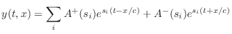
The state of an ideal string at
time ![]() is classically specified by its displacement
is classically specified by its displacement ![]() and
velocity
and
velocity

![$\displaystyle \left[\begin{array}{c} y(t,x) \\ [2pt] v(t,x) \end{array}\right] ...
...ght]
\left[\begin{array}{c} y_r(t-x/c) \\ [2pt] y_l(t+x/c) \end{array}\right].
$](http://www.dsprelated.com/josimages_new/pasp/img3273.png)
![$\displaystyle \left[\begin{array}{c} y'^{+} \\ [2pt] y'^{-} \end{array}\right] ...
...eft[\begin{array}{c} y'-\frac{v}{c} \\ [2pt] y'+\frac{v}{c} \end{array}\right]
$](http://www.dsprelated.com/josimages_new/pasp/img3274.png)
![$\displaystyle \left[\begin{array}{c} y^{+} \\ [2pt] y^{-} \end{array}\right] \eqsp \frac{1}{2}\left[\begin{array}{c} y-w \\ [2pt] y+w \end{array}\right]
$](http://www.dsprelated.com/josimages_new/pasp/img3275.png)
It will be seen in §C.7.4 that state conversion between physical variables and traveling-wave components is simpler when force and velocity are chosen as the physical state variables (as opposed to displacement and velocity used here).
Sampled Traveling Waves
To carry the traveling-wave solution into the ``digital domain,'' it
is necessary to sample the traveling-wave amplitudes at
intervals of ![]() seconds, corresponding to a sampling rate
seconds, corresponding to a sampling rate
![]() samples per second. For CD-quality audio, we have
samples per second. For CD-quality audio, we have
![]() kHz. The natural choice of spatial sampling
interval
kHz. The natural choice of spatial sampling
interval ![]() is the distance sound propagates in one temporal
sampling interval
is the distance sound propagates in one temporal
sampling interval ![]() , or
, or
![]() meters. In a lossless
traveling-wave simulation, the whole wave moves left or right one
spatial sample each time sample; hence, lossless simulation requires
only digital delay lines. By lumping losses parsimoniously in a real
acoustic model, most of the traveling-wave simulation can in fact be
lossless even in a practical application.
meters. In a lossless
traveling-wave simulation, the whole wave moves left or right one
spatial sample each time sample; hence, lossless simulation requires
only digital delay lines. By lumping losses parsimoniously in a real
acoustic model, most of the traveling-wave simulation can in fact be
lossless even in a practical application.
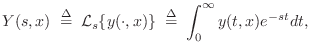
Formally, sampling is carried out by the change of variables
Since
This new notation also introduces a ``
Digital Waveguide Model
![\includegraphics[scale=0.9]{eps/fideal}](http://www.dsprelated.com/josimages_new/pasp/img3287.png) |
In this section, we interpret the sampled d'Alembert traveling-wave solution of the ideal wave equation as a digital filtering framework. This is an example of what are generally known as digital waveguide models [430,431,433,437,442].
The term
![]() in Eq.
in Eq.![]() (C.16) can
be thought of as the output of an
(C.16) can
be thought of as the output of an ![]() -sample delay line whose input is
-sample delay line whose input is
![]() . In general, subtracting a positive number
. In general, subtracting a positive number ![]() from a time
argument
from a time
argument ![]() corresponds to delaying the waveform by
corresponds to delaying the waveform by ![]() samples. Since
samples. Since ![]() is the right-going component, we draw its delay
line with input
is the right-going component, we draw its delay
line with input ![]() on the left and its output
on the left and its output
![]() on the
right. This can be seen as the upper ``rail'' in Fig.C.3
on the
right. This can be seen as the upper ``rail'' in Fig.C.3
Similarly, the term
![]() can be
thought of as the input to an
can be
thought of as the input to an ![]() -sample delay line whose
output is
-sample delay line whose
output is ![]() . Adding
. Adding ![]() to the time argument
to the time argument ![]() produces an
produces an ![]() -sample waveform
advance. Since
-sample waveform
advance. Since ![]() is the left-going component, it makes
sense to draw the delay line with its input
is the left-going component, it makes
sense to draw the delay line with its input
![]() on the right
and its output
on the right
and its output ![]() on the left.
This can be seen as the lower ``rail'' in Fig.C.3.
on the left.
This can be seen as the lower ``rail'' in Fig.C.3.
Note that the position along the string,
![]() meters,
is laid out from left to right in the diagram, giving a physical
interpretation to the horizontal direction in the diagram. Finally,
the left- and right-going traveling waves must be summed to produce a
physical output according to the formula
meters,
is laid out from left to right in the diagram, giving a physical
interpretation to the horizontal direction in the diagram. Finally,
the left- and right-going traveling waves must be summed to produce a
physical output according to the formula
We may compute the physical string displacement at any spatial sampling point
Any ideal, one-dimensional waveguide can be simulated in this way. It
is important to note that the simulation is exact at the
sampling instants, to within the numerical precision of the samples
themselves. To avoid aliasing associated with sampling, we
require all waveshapes traveling along the string to be initially
bandlimited to less than half the sampling frequency. In other
words, the highest frequencies present in the signals ![]() and
and
![]() may not exceed half the temporal sampling frequency
may not exceed half the temporal sampling frequency
![]() ; equivalently, the highest spatial
frequencies in the shapes
; equivalently, the highest spatial
frequencies in the shapes ![]() and
and ![]() may not exceed
half the spatial sampling frequency
may not exceed
half the spatial sampling frequency
![]() .
.
A C program implementing a plucked/struck string model in the form of Fig.C.3 is available at http://ccrma.stanford.edu/~jos/pmudw/.
Digital Waveguide Interpolation
A more compact simulation diagram which stands for either sampled or
continuous waveguide simulation is shown in Fig.C.4.
The figure emphasizes that the ideal, lossless waveguide is simulated
by a bidirectional delay line, and that bandlimited
spatial interpolation may be used to construct a displacement
output for an arbitrary ![]() not a multiple of
not a multiple of ![]() , as suggested by
the output drawn in Fig.C.4. Similarly, bandlimited
interpolation across time serves to evaluate the waveform at an
arbitrary time not an integer multiple of
, as suggested by
the output drawn in Fig.C.4. Similarly, bandlimited
interpolation across time serves to evaluate the waveform at an
arbitrary time not an integer multiple of ![]() (§4.4).
(§4.4).
![\includegraphics[scale=0.9]{eps/fcompact}](http://www.dsprelated.com/josimages_new/pasp/img3301.png)
Ideally, bandlimited interpolation is carried out by convolving a
continuous ``sinc function''
sinc![]() with the signal samples. Specifically, convolving a sampled signal
with the signal samples. Specifically, convolving a sampled signal
![]() with
sinc
with
sinc![]() ``evaluates'' the signal at an
arbitrary continuous time
``evaluates'' the signal at an
arbitrary continuous time ![]() . The sinc function is the impulse
response of the ideal lowpass filter which cuts off at half the
sampling rate.
. The sinc function is the impulse
response of the ideal lowpass filter which cuts off at half the
sampling rate.
In practice, the interpolating sinc function must be windowed
to a finite duration. This means the associated lowpass filter must
be granted a ``transition band'' in which its frequency response is
allowed to ``roll off'' to zero at half the sampling rate. The
interpolation quality in the ``pass band'' can always be made perfect
to within the resolution of human hearing by choosing a sufficiently
large product of window-length times transition-bandwidth. Given
``audibly perfect'' quality in the pass band, increasing the
transition bandwidth reduces the computational expense of the
interpolation. In fact, they are approximately inversely
proportional. This is one reason why oversampling at rates
higher than twice the highest audio frequency is helpful. For
example, at a ![]() kHz sampling rate, the transition bandwidth above
the nominal audio upper limit of
kHz sampling rate, the transition bandwidth above
the nominal audio upper limit of ![]() kHz is only
kHz is only ![]() kHz, while at
a
kHz, while at
a ![]() kHz sampling rate (used in DAT machines) the guard band is
kHz sampling rate (used in DAT machines) the guard band is ![]() kHz wide--nearly double. Since the required window length (impulse
response duration) varies inversely with the provided transition
bandwidth, we see that increasing the sampling rate by less than ten
percent reduces the filter expense by almost fifty percent.
Windowed-sinc interpolation is described further in
§4.4. Many more techniques for digital resampling
and delay-line interpolation are reviewed in
[267].
kHz wide--nearly double. Since the required window length (impulse
response duration) varies inversely with the provided transition
bandwidth, we see that increasing the sampling rate by less than ten
percent reduces the filter expense by almost fifty percent.
Windowed-sinc interpolation is described further in
§4.4. Many more techniques for digital resampling
and delay-line interpolation are reviewed in
[267].
Relation to the Finite Difference Recursion
In this section we will show that the digital waveguide simulation technique is equivalent to the recursion produced by the finite difference approximation (FDA) applied to the wave equation [442, pp. 430-431]. A more detailed derivation, with examples and exploration of implications, appears in Appendix E. Recall from (C.6) that the time update recursion for the ideal string digitized via the FDA is given by
| (C.18) |
To compare this with the waveguide description, we substitute the traveling-wave decomposition
| (C.19) | |||
Thus, we obtain the result that the FDA recursion is also exact in the lossless case, because it is equivalent to the digital waveguide method which we know is exact at the sampling points. This is surprising since the FDA introduces artificial damping when applied to lumped, mass-spring systems, as discussed earlier.
The last identity above can be rewritten as
| (C.20) | |||
which says the displacement at time
This results extends readily to the digital waveguide mesh (§C.14), which is essentially a lattice-work of digital waveguides for simulating membranes and volumes. The equivalence is important in higher dimensions because the finite-difference model requires less computations per node than the digital waveguide approach.
Even in one dimension, the digital waveguide and finite-difference
methods have unique advantages in particular situations, and as a
result they are often combined together to form a hybrid
traveling-wave/physical-variable simulation
[351,352,222,124,123,224,263,223].
In this hybrid simulations, the traveling-wave variables are called
``W variables'' (where `W' stands for ``Wave''), while the physical
variables are caled ``K variables'' (where `K' stands for
``Kirchoff''). Each K variable, such as displacement ![]() on a vibrating string, can be regarded as the sum of two
traveling-wave components, or W variables:
on a vibrating string, can be regarded as the sum of two
traveling-wave components, or W variables:
A Lossy 1D Wave Equation
In any real vibrating string, there are energy losses due to yielding
terminations, drag by the surrounding air, and internal friction within the
string. While losses in solids generally vary in a complicated way with
frequency, they can usually be well approximated by a small number of
odd-order terms added to the wave equation. In the simplest case, force is
directly proportional to transverse string velocity, independent of
frequency. If this proportionality constant is ![]() , we obtain the
modified wave equation
, we obtain the
modified wave equation
Thus, the wave equation has been extended by a ``first-order'' term, i.e., a term proportional to the first derivative of
Setting
![]() in the wave equation to find the relationship
between temporal and spatial frequencies in the eigensolution, the wave
equation becomes
in the wave equation to find the relationship
between temporal and spatial frequencies in the eigensolution, the wave
equation becomes
 |
|||
 |
where
 |
(C.22) |
by the binomial theorem. For this small-loss approximation, we obtain the following relationship between temporal and spatial frequency:
| (C.23) |
The eigensolution is then
| (C.24) |
The right-going part of the eigensolution is
| (C.25) |
which decays exponentially in the direction of propagation, and the left-going solution is
| (C.26) |
which also decays exponentially in the direction of travel.
Setting ![]() and using superposition to build up arbitrary traveling
wave shapes, we obtain the general class of solutions
and using superposition to build up arbitrary traveling
wave shapes, we obtain the general class of solutions
| (C.27) |
Sampling these exponentially decaying traveling waves at intervals of
![]() seconds (or
seconds (or ![]() meters) gives
meters) gives
The simulation diagram for the lossy digital waveguide is shown in Fig.C.5.
![\includegraphics[scale=0.9]{eps/floss}](http://www.dsprelated.com/josimages_new/pasp/img3340.png)
Again the discrete-time simulation of the decaying traveling-wave solution
is an exact implementation of the continuous-time solution at the
sampling positions and instants, even though losses are admitted in the
wave equation. Note also that the losses which are distributed in
the continuous solution have been consolidated, or lumped, at
discrete intervals of ![]() meters in the simulation. The loss factor
meters in the simulation. The loss factor
![]() summarizes the distributed loss incurred in one
sampling interval. The lumping of distributed losses does not introduce
an approximation error at the sampling points. Furthermore, bandlimited
interpolation can yield arbitrarily accurate reconstruction between
samples. The only restriction is again that all initial conditions and
excitations be bandlimited to below half the sampling rate.
summarizes the distributed loss incurred in one
sampling interval. The lumping of distributed losses does not introduce
an approximation error at the sampling points. Furthermore, bandlimited
interpolation can yield arbitrarily accurate reconstruction between
samples. The only restriction is again that all initial conditions and
excitations be bandlimited to below half the sampling rate.
Loss Consolidation
In many applications, it is possible to realize vast computational savings
in digital waveguide models by commuting losses out of unobserved and
undriven sections of the medium and consolidating them at a minimum number
of points. Because the digital simulation is linear and time invariant
(given constant medium parameters
![]() ), and because linear,
time-invariant elements commute, the diagram in Fig.C.6 is
exactly equivalent (to within numerical precision) to the previous diagram
in Fig.C.5.
), and because linear,
time-invariant elements commute, the diagram in Fig.C.6 is
exactly equivalent (to within numerical precision) to the previous diagram
in Fig.C.5.
![\includegraphics[scale=0.9]{eps/flloss}](http://www.dsprelated.com/josimages_new/pasp/img3343.png) |
Frequency-Dependent Losses
In nearly all natural wave phenomena, losses increase with frequency. Distributed losses due to air drag and internal bulk losses in the string tend to increase monotonically with frequency. Similarly, air absorption increases with frequency, adding loss for sound waves in acoustic tubes or open air [318].
Perhaps the apparently simplest modification to Eq.![]() (C.21) yielding
frequency-dependent damping is to add a third-order
time-derivative term [392]:
(C.21) yielding
frequency-dependent damping is to add a third-order
time-derivative term [392]:
While this model has been successful in practice [77], it turns out to go unstable at very high sampling rates. The technical term for this problem is that the PDE is ill posed [45].
A well posed replacement for Eq.![]() (C.28) is given by
(C.28) is given by
in which the third-order partial derivative with respect to time,
The solution of a lossy wave equation containing higher odd-order
derivatives with respect to time yields traveling waves which
propagate with frequency-dependent attenuation. Instead of scalar
factors ![]() distributed throughout the diagram as in Fig.C.5,
each
distributed throughout the diagram as in Fig.C.5,
each ![]() factor becomes a lowpass filter having some
frequency-response per sample denoted by
factor becomes a lowpass filter having some
frequency-response per sample denoted by ![]() . Because
propagation is passive, we will always have
. Because
propagation is passive, we will always have
![]() .
.
More specically, As shown in [392], odd-order partial derivatives with respect to time in the wave equation of the form

In view of the above, we see that we can add odd-order time
derivatives to the wave equation to approximate experimentally
observed frequency-dependent damping characteristics in vibrating
strings [73]. However, we then have the problem that
such wave equations are ill posed, leading to possible stability
failures at high sampling rates. As a result, it is generally
preferable to use mixed derivatives, as in Eq.![]() (C.29), and try to
achieve realistic damping using higher order spatial derivatives
instead.
(C.29), and try to
achieve realistic damping using higher order spatial derivatives
instead.
Well Posed PDEs for Modeling Damped Strings
A large class of well posed PDEs is given by [45]
Thus, to the ideal string wave equation Eq.
Digital Filter Models of Damped Strings
In an efficient digital simulation, lumped loss factors of the form
![]() are approximated by a rational frequency response
are approximated by a rational frequency response
![]() . In general, the coefficients of the optimal rational
loss filter are obtained by minimizing
. In general, the coefficients of the optimal rational
loss filter are obtained by minimizing
![]() with respect to the filter coefficients or the poles
and zeros of the filter. To avoid introducing frequency-dependent
delay, the loss filter should be a zero-phase,
finite-impulse-response (FIR) filter [362].
Restriction to zero phase requires the impulse response
with respect to the filter coefficients or the poles
and zeros of the filter. To avoid introducing frequency-dependent
delay, the loss filter should be a zero-phase,
finite-impulse-response (FIR) filter [362].
Restriction to zero phase requires the impulse response
![]() to
be finite in length (i.e., an FIR filter) and it must be symmetric
about time zero, i.e.,
to
be finite in length (i.e., an FIR filter) and it must be symmetric
about time zero, i.e.,
![]() . In most implementations,
the zero-phase FIR filter can be converted into a causal, linear
phase filter by reducing an adjacent delay line by half of the
impulse-response duration.
. In most implementations,
the zero-phase FIR filter can be converted into a causal, linear
phase filter by reducing an adjacent delay line by half of the
impulse-response duration.
Lossy Finite Difference Recursion
We will now derive a finite-difference model in terms of string displacement samples which correspond to the lossy digital waveguide model of Fig.C.5. This derivation generalizes the lossless case considered in §C.4.3.
Figure C.7 depicts a digital waveguide section once again in ``physical canonical form,'' as shown earlier in Fig.C.5, and introduces a doubly indexed notation for greater clarity in the derivation below [442,222,124,123].
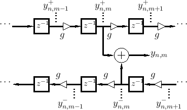
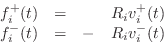
Referring to Fig.C.7, we have the following time-update relations:
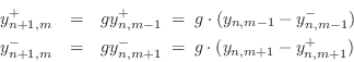
Adding these equations gives
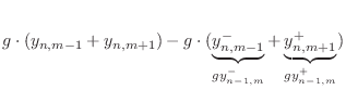
This is now in the form of the finite-difference time-domain (FDTD) scheme analyzed in [222]:
Frequency-Dependent Losses
The preceding derivation generalizes immediately to
frequency-dependent losses. First imagine each ![]() in Fig.C.7
to be replaced by
in Fig.C.7
to be replaced by ![]() , where for passivity we require
, where for passivity we require
![\begin{eqnarray*}
y^{+}_{n+1,m}&=& g\ast y^{+}_{n,m-1}\;=\; g\ast (y_{n,m-1}- y^...
...
&=& g\ast \left[(y_{n,m-1}+y_{n,m+1}) - g\ast y_{n-1,m}\right]
\end{eqnarray*}](http://www.dsprelated.com/josimages_new/pasp/img3373.png)
where ![]() denotes convolution (in the time dimension only).
Define filtered node variables by
denotes convolution (in the time dimension only).
Define filtered node variables by

Then the frequency-dependent FDTD scheme is simply
The frequency-dependent generalization of the FDTD scheme described in this section extends readily to the digital waveguide mesh. See §C.14.5 for the outline of the derivation.
The Dispersive 1D Wave Equation
In the ideal vibrating string, the only restoring force for transverse displacement comes from the string tension (§C.1 above); specifically, the transverse restoring force is equal the net transverse component of the axial string tension. Consider in place of the ideal string a bundle of ideal strings, such as a stranded cable. When the cable is bent, there is now a new restoring force arising from some of the fibers being compressed and others being stretched by the bending. This force sums with that due to string tension. Thus, stiffness in a vibrating string introduces a new restoring force proportional to bending angle. It is important to note that string stiffness is a linear phenomenon resulting from the finite diameter of the string.
In typical treatments,C.3bending stiffness adds a new term to the wave equation that is proportional to the fourth spatial derivative of string displacement:
where the moment constant
To solve the stiff wave equation Eq.![]() (C.32),
we may set
(C.32),
we may set
![]() to get
to get
At very high frequencies, or when the tension ![]() is negligible relative
to
is negligible relative
to
![]() , we obtain the ideal bar (or rod) approximation:
, we obtain the ideal bar (or rod) approximation:
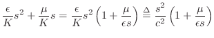
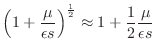
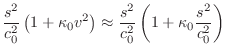
At intermediate frequencies, between the ideal string and the ideal bar,
the stiffness contribution can be treated as a correction term
[95]. This is the region of most practical interest because
it is the principal operating region for strings, such as piano strings,
whose stiffness has audible consequences (an inharmonic, stretched overtone
series). Assuming
![]() ,
,
 |
|||
 |
|||
 |
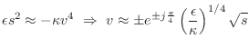
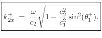
Substituting for
![$\displaystyle e^{st+vx} = \exp{\left\{{s\left[t\pm \frac{x}{c_0}\left(
1+\frac{1}{2}\kappa_0 \frac{s^2}{c_0^2} \right)\right]}\right\}}.
$](http://www.dsprelated.com/josimages_new/pasp/img3398.png)
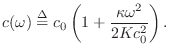
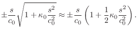
Since the temporal and spatial sampling intervals are related by ![]() , this must generalize to
, this must generalize to
![]() , where
, where ![]() is the size of a unit
delay in the absence of stiffness. Thus, a unit delay
is the size of a unit
delay in the absence of stiffness. Thus, a unit delay ![]() may be
replaced by
may be
replaced by
![\includegraphics[scale=0.9]{eps/fstiffstring}](http://www.dsprelated.com/josimages_new/pasp/img3406.png)
The general, order ![]() , allpass filter is given by [449]
, allpass filter is given by [449]
For computability of the string simulation in the presence of scattering
junctions, there must be at least one sample of pure delay along each
uniform section of string. This means for at least one allpass filter in
Fig.C.8, we must have
![]() which
implies
which
implies ![]() can be factored as
can be factored as
![]() . In a
systolic VLSI implementation, it is desirable to have at least one real
delay from the input to the output of every allpass filter, in order
to be able to pipeline the computation of all of the allpass filters in
parallel. Computability can be arranged in practice by deciding on a
minimum delay, (e.g., corresponding to the wave velocity at a maximum
frequency), and using an allpass filter to provide excess delay beyond the
minimum.
. In a
systolic VLSI implementation, it is desirable to have at least one real
delay from the input to the output of every allpass filter, in order
to be able to pipeline the computation of all of the allpass filters in
parallel. Computability can be arranged in practice by deciding on a
minimum delay, (e.g., corresponding to the wave velocity at a maximum
frequency), and using an allpass filter to provide excess delay beyond the
minimum.
Because allpass filters are linear and time invariant, they commute
like gain factors with other linear, time-invariant components.
Fig.C.9 shows a diagram equivalent to
Fig.C.8 in which the allpass filters have been
commuted and consolidated at two points. For computability in all
possible contexts (e.g., when looped on itself), a single sample of
delay is pulled out along each rail. The remaining transfer function,
![]() in the example of
Fig.C.9, can be approximated using any allpass filter
design technique
[1,2,267,272,551].
Alternatively, both gain and dispersion for a stretch of waveguide can
be provided by a single filter which can be designed using any
general-purpose filter design method which is sensitive to
frequency-response phase as well as magnitude; examples include
equation error methods (such as used in the matlab invfreqz
function (§8.6.4), and Hankel norm methods
[177,428,36].
in the example of
Fig.C.9, can be approximated using any allpass filter
design technique
[1,2,267,272,551].
Alternatively, both gain and dispersion for a stretch of waveguide can
be provided by a single filter which can be designed using any
general-purpose filter design method which is sensitive to
frequency-response phase as well as magnitude; examples include
equation error methods (such as used in the matlab invfreqz
function (§8.6.4), and Hankel norm methods
[177,428,36].
![\includegraphics[scale=0.9]{eps/flstiffstring}](http://www.dsprelated.com/josimages_new/pasp/img3413.png) |
In the case of a lossless, stiff string, if ![]() denotes the
consolidated allpass transfer function, it can be argued that the filter
design technique used should minimize the phase-delay error, where
phase delay is defined by [362]
denotes the
consolidated allpass transfer function, it can be argued that the filter
design technique used should minimize the phase-delay error, where
phase delay is defined by [362]
 (Phase Delay)
Alternatively, a lumped allpass filter can be designed by minimizing group delay,
 (Group Delay)
See §9.4.1 for designing allpass filters with a prescribed delay versus frequency. To model stiff strings, the allpass filter must supply a phase delay which decreases as frequency increases. A good approximation may require a fairly high-order filter, adding significantly to the cost of simulation. (For low-pitched piano strings, order 8 allpass filters work well perceptually [1].) To a large extent, the allpass order required for a given error tolerance increases as the number of lumped frequency-dependent delays is increased. Therefore, increased dispersion consolidation is accompanied by larger required allpass filters, unlike the case of resistive losses.
The function piano_dispersion_filter in the Faust distribution (in effect.lib) designs and implements an allpass filter modeling the dispersion due to stiffness in a piano string [154,170,368].
Higher Order Terms
The complete, linear, time-invariant generalization of the lossy, stiff string is described by the differential equation

which, on setting
 |
(C.34) |
Solving for
| (C.35) | |||
where
We see that a large class of wave equations with constant coefficients, of any order, admits a decaying, dispersive, traveling-wave type solution. Even-order time derivatives give rise to frequency-dependent dispersion and odd-order time derivatives correspond to frequency-dependent losses. The corresponding digital simulation of an arbitrarily long (undriven and unobserved) section of medium can be simplified via commutativity to at most two pure delays and at most two linear, time-invariant filters.
Every linear, time-invariant filter can be expressed as a zero-phase filter in series with an allpass filter. The zero-phase part can be interpreted as implementing a frequency-dependent gain (damping in a digital waveguide), and the allpass part can be seen as frequency-dependent delay (dispersion in a digital waveguide).
Alternative Wave Variables
We have thus far considered discrete-time simulation of transverse
displacement ![]() in the ideal string. It is equally valid to
choose velocity
in the ideal string. It is equally valid to
choose velocity
![]() , acceleration
, acceleration
![]() , slope
, slope ![]() , or perhaps some other derivative
or integral of displacement with respect to time or position.
Conversion between various time derivatives can be carried out by
means integrators and differentiators, as depicted in
Fig.C.10. Since integration and
differentiation are linear operators, and since the traveling
wave arguments are in units of time, the conversion formulas relating
, or perhaps some other derivative
or integral of displacement with respect to time or position.
Conversion between various time derivatives can be carried out by
means integrators and differentiators, as depicted in
Fig.C.10. Since integration and
differentiation are linear operators, and since the traveling
wave arguments are in units of time, the conversion formulas relating
![]() ,
, ![]() , and
, and ![]() hold also for the traveling wave components
hold also for the traveling wave components
![]() .
.
![\includegraphics[scale=0.9]{eps/fwaveconversions}](http://www.dsprelated.com/josimages_new/pasp/img3445.png) |
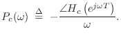
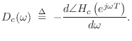
Differentiation and integration have a simple form in the
frequency domain. Denoting the Laplace Transform of ![]() by
by
 |
(C.36) |
where ``
| (C.37) |
Similarly,
![\includegraphics[scale=0.9]{eps/ffdwaveconversions}](http://www.dsprelated.com/josimages_new/pasp/img3449.png)
In discrete time, integration and differentiation can be accomplished using digital filters [362]. Commonly used first-order approximations are shown in Fig.C.12.
![\includegraphics[width=\twidth]{eps/fdigitaldiffint}](http://www.dsprelated.com/josimages_new/pasp/img3450.png) |
If discrete-time acceleration ![]() is defined as the sampled version of
continuous-time acceleration, i.e.,
is defined as the sampled version of
continuous-time acceleration, i.e.,
![]() , (for some fixed continuous position
, (for some fixed continuous position ![]() which we
suppress for simplicity of notation), then the
frequency-domain form is given by the
which we
suppress for simplicity of notation), then the
frequency-domain form is given by the ![]() transform
[485]:
transform
[485]:
 |
(C.38) |
In the frequency domain for discrete-time systems, the first-order approximate conversions appear as shown in Fig.C.13.
![\includegraphics[scale=0.6]{eps/ffddigitaldiffint}](http://www.dsprelated.com/josimages_new/pasp/img3454.png) |
The ![]() transform plays the role of the Laplace transform for discrete-time
systems. Setting
transform plays the role of the Laplace transform for discrete-time
systems. Setting ![]() , it can be seen as a sampled Laplace
transform (divided by
, it can be seen as a sampled Laplace
transform (divided by ![]() ), where the sampling is carried out by halting
the limit of the rectangle width at
), where the sampling is carried out by halting
the limit of the rectangle width at ![]() in the definition of a Reimann
integral for the Laplace transform. An important difference between the
two is that the frequency axis in the Laplace transform is the imaginary
axis (the ``
in the definition of a Reimann
integral for the Laplace transform. An important difference between the
two is that the frequency axis in the Laplace transform is the imaginary
axis (the ``![]() axis''), while the frequency axis in the
axis''), while the frequency axis in the ![]() plane is on
the unit circle
plane is on
the unit circle
![]() . As one would expect, the frequency axis for
discrete-time systems has unique information only between frequencies
. As one would expect, the frequency axis for
discrete-time systems has unique information only between frequencies
![]() and
and ![]() while the continuous-time frequency axis extends to plus and
minus infinity.
while the continuous-time frequency axis extends to plus and
minus infinity.
These first-order approximations are accurate (though scaled by ![]() )
at low frequencies relative to half the sampling rate, but they are
not ``best'' approximations in any sense other than being most like
the definitions of integration and differentiation in continuous time.
Much better approximations can be obtained by approaching the problem
from a digital filter design viewpoint, as discussed in §8.6.
)
at low frequencies relative to half the sampling rate, but they are
not ``best'' approximations in any sense other than being most like
the definitions of integration and differentiation in continuous time.
Much better approximations can be obtained by approaching the problem
from a digital filter design viewpoint, as discussed in §8.6.
Spatial Derivatives
In addition to time derivatives, we may apply any number of spatial
derivatives to obtain yet more wave variables to choose from. The first
spatial derivative of string displacement yields slope waves

or, in discrete time,
From this we may conclude that
By the wave equation, curvature waves,
![]() , are
simply a scaling of acceleration waves, in the case of ideal strings.
, are
simply a scaling of acceleration waves, in the case of ideal strings.
In the field of acoustics, the state of a vibrating string at any
instant of time ![]() is often specified by the displacement
is often specified by the displacement
![]() and velocity
and velocity
![]() for all
for all ![]() [317]. Since
velocity is the sum of the traveling velocity waves and
displacement is determined by the difference of the
traveling velocity waves, viz., from Eq.
[317]. Since
velocity is the sum of the traveling velocity waves and
displacement is determined by the difference of the
traveling velocity waves, viz., from Eq.![]() (C.39),
(C.39),
![$\displaystyle y(t,x) \eqsp \int_0^{x} y'(t,\xi)d\xi
\eqsp -\frac{1}{c}\int_0^{x} \left[v_r(t-\xi/c) - v_l(t+\xi/c)\right]d\xi,
$](http://www.dsprelated.com/josimages_new/pasp/img3474.png)
In summary, all traveling-wave variables can be computed from any one, as long as both the left- and right-going component waves are available. Alternatively, any two linearly independent physical variables, such as displacement and velocity, can be used to compute all other wave variables. Wave variable conversions requiring differentiation or integration are relatively expensive since a large-order digital filter is necessary to do it right (§8.6.1). Slope and velocity waves can be computed from each other by simple scaling, and curvature waves are identical to acceleration waves to within a scale factor.
In the absence of factors dictating a specific choice, velocity waves are a good overall choice because (1) it is numerically easier to perform digital integration to get displacement than it is to differentiate displacement to get velocity, (2) slope waves are immediately computable from velocity waves. Slope waves are important because they are a simple scaling of force waves.
Force Waves
![\includegraphics[width=\twidth]{eps/fStringForce}](http://www.dsprelated.com/josimages_new/pasp/img3475.png)
Referring to Fig.C.14, at an arbitrary point ![]() along
the string, the vertical force applied at time
along
the string, the vertical force applied at time ![]() to the portion of
string to the left of position
to the portion of
string to the left of position ![]() by the portion of string to the
right of position
by the portion of string to the
right of position ![]() is given by
is given by
| (C.41) |
assuming
| (C.42) |
These forces must cancel since a nonzero net force on a massless point would produce infinite acceleration. I.e., we must have
Vertical force waves propagate along the string like any other
transverse wave variable (since they are just slope waves multiplied
by tension ![]() ). We may choose either
). We may choose either ![]() or
or ![]() as the string
force wave variable, one being the negative of the other. It turns
out that to make the description for vibrating strings look the same
as that for air columns, we have to pick
as the string
force wave variable, one being the negative of the other. It turns
out that to make the description for vibrating strings look the same
as that for air columns, we have to pick ![]() , the one that
acts to the right. This makes sense intuitively when one
considers longitudinal pressure waves in an acoustic tube: a
compression wave traveling to the right in the tube pushes the air in
front of it and thus acts to the right. We therefore define the
force wave variable to be
, the one that
acts to the right. This makes sense intuitively when one
considers longitudinal pressure waves in an acoustic tube: a
compression wave traveling to the right in the tube pushes the air in
front of it and thus acts to the right. We therefore define the
force wave variable to be
| (C.43) |
Note that a negative slope pulls up on the segment to the right. At this point, we have not yet considered a traveling-wave decomposition.
Wave Impedance
Using the above identities, we have that the force distribution along the string is given in terms of velocity waves by
![$\displaystyle f(t,x) = \frac{K}{c} \left[{\dot y}_r(t-x/c) - {\dot y}_l(t+x/c) \right], \protect$](http://www.dsprelated.com/josimages_new/pasp/img3483.png)
where
 |
(C.45) |
The wave impedance can be seen as the geometric mean of the two resistances to displacement: tension (spring force) and mass (inertial force).
The digitized traveling force-wave components become
which gives us that the right-going force wave equals the wave impedance times the right-going velocity wave, and the left-going force wave equals minus the wave impedance times the left-going velocity wave.C.4Thus, in a traveling wave, force is always in phase with velocity (considering the minus sign in the left-going case to be associated with the direction of travel rather than a
In the case of the acoustic tube [317,297], we have the analogous relations
 |
(C.47) |
where
| (C.48) |
where
State Conversions
In §C.3.6, an arbitrary string state was converted to traveling displacement-wave components to show that the traveling-wave representation is complete, i.e., that any physical string state can be expressed as a pair of traveling-wave components. In this section, we revisit this topic using force and velocity waves.
By definition of the traveling-wave decomposition, we have
Using Eq.![]() (C.46), we can eliminate
(C.46), we can eliminate
![]() and
and
![]() ,
giving, in matrix form,
,
giving, in matrix form,
![$\displaystyle \left[\begin{array}{c} f \\ [2pt] v \end{array}\right] = \left[\b...
...ay}\right]
\left[\begin{array}{c} f^{{+}} \\ [2pt] f^{{-}} \end{array}\right].
$](http://www.dsprelated.com/josimages_new/pasp/img3492.png)
![$\displaystyle \left[\begin{array}{c} f \\ [2pt] v \end{array}\right] = \left[\b...
...d{array}\right]\left[\begin{array}{c} v^{+} \\ [2pt] v^{-} \end{array}\right].
$](http://www.dsprelated.com/josimages_new/pasp/img3494.png)
Carrying out the inversion to obtain force waves
![]() from
from
![]() yields
yields
![$\displaystyle \left[\begin{array}{c} f^{{+}} \\ [2pt] f^{{-}} \end{array}\right...
...ft[\begin{array}{c} \frac{f+Rv}{2} \\ [2pt] \frac{f-Rv}{2} \end{array}\right].
$](http://www.dsprelated.com/josimages_new/pasp/img3498.png)
![$\displaystyle \left[\begin{array}{c} v^{+} \\ [2pt] v^{-} \end{array}\right] = ...
...[\begin{array}{c} \frac{v+f/R}{2} \\ [2pt] \frac{v-f/R}{2} \end{array}\right].
$](http://www.dsprelated.com/josimages_new/pasp/img3500.png)
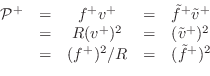
Power Waves
Basic courses in physics teach us that power is work per unit time, and work is a measure of energy which is typically defined as force times distance. Therefore, power is in physical units of force times distance per unit time, or force times velocity. It therefore should come as no surprise that traveling power waves are defined for strings as follows:
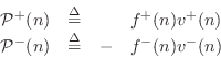 |
From the Ohm's-law relations
![\begin{eqnarray*}
{\cal P}^{+}(n)&=&R[v^{+}(n)]^2 \eqsp [f^{{+}}(n)]^2/R,
\\
{\cal P}^{-}(n)&=&R[v^{-}(n)]^2 \eqsp [f^{{-}}(n)]^2/R.
\end{eqnarray*}](http://www.dsprelated.com/josimages_new/pasp/img3502.png)
Thus, both the left- and right-going components are nonnegative. The sum of the traveling powers at a point gives the total power at that point in the waveguide:
| (C.49) |
If we had left out the minus sign in the definition of left-going power waves, the sum would instead be a net power flow.
Power waves are important because they correspond to the actual ability of the wave to do work on the outside world, such as on a violin bridge at the end of a string. Because energy is conserved in closed systems, power waves sometimes give a simpler, more fundamental view of wave phenomena, such as in conical acoustic tubes. Also, implementing nonlinear operations such as rounding and saturation in such a way that signal power is not increased, gives suppression of limit cycles and overflow oscillations [432], as discussed in the section on signal scattering.
For example, consider a waveguide having a wave impedance which
increases smoothly to the right. A converging cone provides a
practical example in the acoustic tube realm. Then since the energy
in a traveling wave must be in the wave unless it has been transduced
elsewhere, we expect
![]() to propagate unchanged along the
waveguide. However, since the wave impedance is increasing, it must
be true that force is increasing and velocity is decreasing according
to
to propagate unchanged along the
waveguide. However, since the wave impedance is increasing, it must
be true that force is increasing and velocity is decreasing according
to
![]() . Looking only at force or velocity
might give us the mistaken impression that the wave is getting
stronger (looking at force) or weaker (looking at velocity), when
really it was simply sailing along as a fixed amount of energy. This
is an example of a transformer action in which force is
converted into velocity or vice versa. It is well known that a
conical tube acts as if it's open on both ends even though we can
plainly see that it is closed on one end. A tempting explanation is
that the cone acts as a transformer which exchanges pressure and
velocity between the endpoints of the tube, so that a closed end on
one side is equivalent to an open end on the other. However, this
view is oversimplified because, while spherical pressure waves travel
nondispersively in cones, velocity propagation is dispersive
[22,50].
. Looking only at force or velocity
might give us the mistaken impression that the wave is getting
stronger (looking at force) or weaker (looking at velocity), when
really it was simply sailing along as a fixed amount of energy. This
is an example of a transformer action in which force is
converted into velocity or vice versa. It is well known that a
conical tube acts as if it's open on both ends even though we can
plainly see that it is closed on one end. A tempting explanation is
that the cone acts as a transformer which exchanges pressure and
velocity between the endpoints of the tube, so that a closed end on
one side is equivalent to an open end on the other. However, this
view is oversimplified because, while spherical pressure waves travel
nondispersively in cones, velocity propagation is dispersive
[22,50].
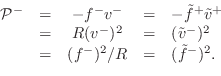
Energy Density Waves
The vibrational energy per unit length along the string, or wave energy density [317] is given by the sum of potential and kinetic energy densities:
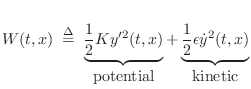 |
(C.50) |
Sampling across time and space, and substituting traveling wave components, one can show in a few lines of algebra that the sampled wave energy density is given by
| (C.51) |
where
![\begin{eqnarray*}
W^{+}(n) &=& \frac{{\cal P}^{+}(n)}{c} \,\mathrel{\mathop=}\,\...
...ht]^2 \,\mathrel{\mathop=}\,\frac{\left[f^{{-}}(n)\right]^2}{K}.
\end{eqnarray*}](http://www.dsprelated.com/josimages_new/pasp/img3508.png)
Thus, traveling power waves (energy per unit time)
can be converted to energy density waves (energy per unit length) by
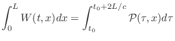
simply dividing by ![]() , the speed of propagation. Quite naturally, the
total wave energy in the string
is given by the integral along the string of the energy density:
, the speed of propagation. Quite naturally, the
total wave energy in the string
is given by the integral along the string of the energy density:
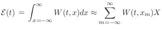 |
(C.52) |
In practice, of course, the string length is finite, and the limits of integration are from the
Root-Power Waves
It is sometimes helpful to normalize the wave variables so that signal power is uniformly distributed numerically. This can be especially helpful in fixed-point implementations.
From (C.49), it is clear that power normalization is given by
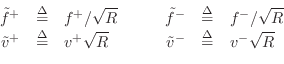
where we have dropped the common time argument `
 |
and
 |
The normalized wave variables
Total Energy in a Rigidly Terminated String
The total energy ![]() in a length
in a length ![]() , rigidly terminated, freely
vibrating string can be computed as
, rigidly terminated, freely
vibrating string can be computed as
 |
(C.54) | ||
 |
(C.55) |
for any
Scattering at Impedance Changes
When a traveling wave encounters a change in wave impedance, scattering occurs, i.e., a traveling wave impinging on an impedance discontinuity will partially reflect and partially transmit at the junction in such a way that energy is conserved. This is a classical topic in transmission line theory [295], and it is well covered for acoustic tubes in a variety of references [297,363]. However, for completeness, we derive the basic scattering relations below for plane waves in air, and for longitudinal stress waves in rods.
Plane-Wave Scattering
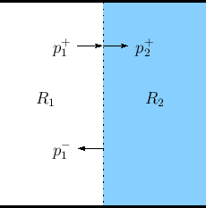
Consider a plane wave with peak pressure amplitude ![]() propagating
from wave impedance
propagating
from wave impedance ![]() into a new wave impedance
into a new wave impedance ![]() , as shown in
Fig.C.15. (Assume
, as shown in
Fig.C.15. (Assume ![]() and
and ![]() are real and positive.)
The physical constraints on the wave are that
are real and positive.)
The physical constraints on the wave are that
- pressure must be continuous everywhere, and
- velocity in must equal velocity out (the junction has no state).
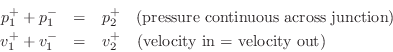
As derived in §C.7.3, we also have the Ohm's law relations:

To obey the physical constraints at the impedance discontinuity, the
incident plane-wave must split into a reflected plane wave
![]() and a transmitted plane-wave
and a transmitted plane-wave ![]() such that
pressure is continuous and signal power is conserved. The physical
pressure on the left of the junction is
such that
pressure is continuous and signal power is conserved. The physical
pressure on the left of the junction is
![]() , and the
physical pressure on the right of the junction is
, and the
physical pressure on the right of the junction is
![]() , since
, since ![]() according to our set-up.
according to our set-up.
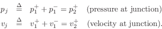
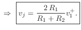
Scattering Solution
Define the junction pressure ![]() and junction velocity
and junction velocity ![]() by
by
Then we can write
![\begin{eqnarray*}
p^+_1+p^-_1 &=& p^+_2\;=\;p_j\\ [10pt]
\,\,\Rightarrow\,\,R_1v...
...\\ [10pt]
\,\,\Rightarrow\,\,2\,R_1v^{+}_1 - R_1 v_j &=& R_2 v_j
\end{eqnarray*}](http://www.dsprelated.com/josimages_new/pasp/img3532.png)
![$\displaystyle v^{-}_1 = v_j - v^{+}_1 = \left[\frac{2\,R_1}{R_1+R_2} - 1\right]v^{+}_1 = \frac{R_1-R_2}{R_1+R_2} v^{+}_1.
$](http://www.dsprelated.com/josimages_new/pasp/img3536.png)
Using the Ohm's law relations, the pressure waves follow easily:
![\begin{eqnarray*}
p^+_2 &=& R_2v^{+}_2 = R_2 v_j = \frac{2\,R_2}{R_1+R_2}p^+_1\\ [10pt]
p^-_1 &=& -R_1v^{-}_1 = \frac{R_2-R_1}{R_1+R_2} p^+_1
\end{eqnarray*}](http://www.dsprelated.com/josimages_new/pasp/img3537.png)
Reflection Coefficient
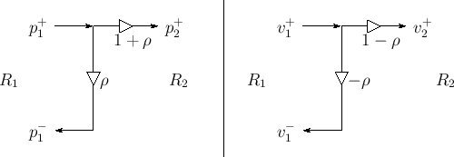
Define the reflection coefficient of the scattering junction as

![\begin{eqnarray*}
p^+_2 &=& (1+\rho)p^+_1\\ [3pt]
p^-_1 &=& \rho\,p^+_1
\end{eqnarray*}](http://www.dsprelated.com/josimages_new/pasp/img3539.png)
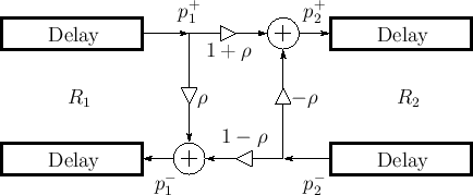
Signal flow graphs for pressure and velocity are given in Fig.C.16.
 |
It is a simple exercise to verify that signal power is conserved by
checking that
![]() .
(Left-going power is negated to account for its opposite
direction-of-travel.)
.
(Left-going power is negated to account for its opposite
direction-of-travel.)
So far we have only considered a plane wave incident on the left of
the junction. Consider now a plane wave incident from the right. For
that wave, the impedance steps from ![]() to
to ![]() , so the reflection
coefficient it ``sees'' is
, so the reflection
coefficient it ``sees'' is ![]() . By superposition, the signal flow
graph for plane waves incident from either side is given by
Fig.C.17. Note that the transmission coefficient is
one plus the reflection coefficient in either direction. This signal
flow graph is often called the ``Kelly-Lochbaum'' scattering junction
[297].
. By superposition, the signal flow
graph for plane waves incident from either side is given by
Fig.C.17. Note that the transmission coefficient is
one plus the reflection coefficient in either direction. This signal
flow graph is often called the ``Kelly-Lochbaum'' scattering junction
[297].
 |
There are some simple special cases:
-
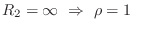 (e.g., rigid wall reflection)
-
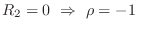 (e.g., open-ended tube)
-
 (no reflection)
Plane-Wave Scattering at an Angle
Figure C.18 shows the more general situation (as compared
to Fig.C.15) of a sinusoidal traveling plane wave
encountering an impedance discontinuity at some arbitrary angle of
incidence, as indicated by the vector wavenumber
![]() . The
mathematical details of general sinusoidal plane waves in air and
vector wavenumber are reviewed in §B.8.1.
. The
mathematical details of general sinusoidal plane waves in air and
vector wavenumber are reviewed in §B.8.1.
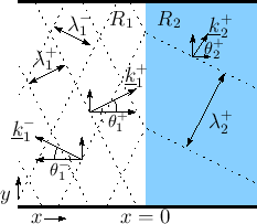 |
At the boundary between impedance ![]() and
and ![]() , we have, by
continuity of pressure,
, we have, by
continuity of pressure,
as we will now derive.
Let the impedance change be in the
![]() plane. Thus, the
impedance is
plane. Thus, the
impedance is ![]() for
for ![]() and
and ![]() for
for ![]() . There are three
plane waves to consider:
. There are three
plane waves to consider:
- The incident plane wave with wave vector

- The reflected plane wave with wave vector

- The transmitted plane wave with wave vector

where
Reflection and Refraction
The first equality in Eq.![]() (C.56) implies that the
angle of incidence equals angle of reflection:
(C.56) implies that the
angle of incidence equals angle of reflection:
We now wish to find the wavenumber in medium 2.
Let ![]() denote the phase velocity in wave impedance
denote the phase velocity in wave impedance ![]() :
:
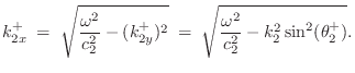
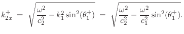
Evanescent Wave due to Total Internal Reflection
Note that if
![]() , the horizontal component
of the wavenumber in medium 2 becomes imaginary. In this case,
the wave in medium 2 is said to be evanescent, and the wave in
medium 1 undergoes total internal reflection (no power travels
from medium 1 to medium 2). The evanescent-wave amplitude decays
exponentially to the right and oscillates ``in place'' (like a
standing wave). ``Tunneling'' is possible given a
medium 3 beyond medium 2 in which wave propagation resumes.
, the horizontal component
of the wavenumber in medium 2 becomes imaginary. In this case,
the wave in medium 2 is said to be evanescent, and the wave in
medium 1 undergoes total internal reflection (no power travels
from medium 1 to medium 2). The evanescent-wave amplitude decays
exponentially to the right and oscillates ``in place'' (like a
standing wave). ``Tunneling'' is possible given a
medium 3 beyond medium 2 in which wave propagation resumes.
To show explicitly the exponential decay and in-place oscillation in
an evanescent wave, express the imaginary wavenumber as
![]() . Then we have
. Then we have
![\begin{eqnarray*}
p(t,\underline{x}) &=&
\cos\left(\omega t - \underline{k}^T\...
...-k_x x}\right\}}}\\ [5pt]
&=& e^{-k_x x} \cos(\omega t - k_y y).
\end{eqnarray*}](http://www.dsprelated.com/josimages_new/pasp/img3576.png)
Thus, an imaginary wavenumber corresponds to an exponentially decaying evanescent wave. Note that the time dependence (cosine term) applies to all points to the right of the boundary. Since evanescent waves do not really ``propagate,'' it is perhaps better to speak of an ``evanescent acoustic field'' or ``evanescent standing wave'' instead of ``evanescent waves''.
For more on the physics of evanescent waves and tunneling, see [295].
Longitudinal Waves in Rods
In this section, elementary scattering relations will be derived for the case of longitudinal force and velocity waves in an ideal string or rod. In solids, force-density waves are referred to as stress waves [169,261]. Longitudinal stress waves in strings and rods have units of (compressive) force per unit area and are analogous to longitudinal pressure waves in acoustic tubes.
![\includegraphics[width=\twidth]{eps/Fwgfs}](http://www.dsprelated.com/josimages_new/pasp/img3577.png) |
A single waveguide section between two partial sections is shown in
Fig.C.19. The sections are numbered 0 through ![]() from
left to right, and their wave impedances are
from
left to right, and their wave impedances are ![]() ,
, ![]() , and
, and ![]() ,
respectively. Such a rod might be constructed, for example, using
three different materials having three different densities. In the
,
respectively. Such a rod might be constructed, for example, using
three different materials having three different densities. In the
![]() th section, there are two stress traveling waves:
th section, there are two stress traveling waves: ![]() traveling
to the right at speed
traveling
to the right at speed ![]() , and
, and ![]() traveling to the left at speed
traveling to the left at speed
![]() . To minimize the numerical dynamic range, velocity waves may be
chosen instead when
. To minimize the numerical dynamic range, velocity waves may be
chosen instead when ![]() .
.
As in the case of transverse waves (see the derivation of (C.46)), the traveling longitudinal plane waves in each section satisfy [169,261]
where the wave impedance is now
If the wave impedance ![]() is constant, the shape of a traveling wave
is not altered as it propagates from one end of a rod-section to the
other. In this case we need only consider
is constant, the shape of a traveling wave
is not altered as it propagates from one end of a rod-section to the
other. In this case we need only consider ![]() and
and ![]() at one
end of each section as a function of time. As shown in Fig.C.19,
we define
at one
end of each section as a function of time. As shown in Fig.C.19,
we define
![]() as the force-wave component at the extreme
left of section
as the force-wave component at the extreme
left of section ![]() . Therefore, at the extreme right of section
. Therefore, at the extreme right of section ![]() ,
we have the traveling waves
,
we have the traveling waves
![]() and
and
![]() , where
, where ![]() is
the travel time from one end of a section to the other.
is
the travel time from one end of a section to the other.
For generality, we may allow the wave impedances ![]() to vary with
time. A number of possibilities exist which satisfy (C.57) in the
time-varying case. For the moment, we will assume the traveling waves
at the extreme right of section
to vary with
time. A number of possibilities exist which satisfy (C.57) in the
time-varying case. For the moment, we will assume the traveling waves
at the extreme right of section ![]() are still given by
are still given by
![]() and
and
![]() . This definition, however, implies the velocity varies
inversely with the wave impedance. As a result, signal energy, being the product
of force times velocity, is ``pumped'' into or out of the waveguide
by a changing wave impedance. Use of normalized waves
. This definition, however, implies the velocity varies
inversely with the wave impedance. As a result, signal energy, being the product
of force times velocity, is ``pumped'' into or out of the waveguide
by a changing wave impedance. Use of normalized waves
![]() avoids this.
However, normalization increases the required number of
multiplications, as we will see in §C.8.6 below.
avoids this.
However, normalization increases the required number of
multiplications, as we will see in §C.8.6 below.
As before, the physical force density (stress) and velocity at the
left end of section ![]() are obtained by summing the left- and
right-going traveling wave components:
are obtained by summing the left- and
right-going traveling wave components:
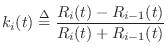
Let
Kelly-Lochbaum Scattering Junctions
Conservation of energy and mass dictate that, at the impedance
discontinuity, force and velocity variables must be continuous
where velocity is defined as positive to the right on both sides of the junction. Force (or stress or pressure) is a scalar while velocity is a vector with both a magnitude and direction (in this case only left or right). Equations (C.57), (C.58), and (C.59) imply the following scattering equations (a derivation is given in the next section for the more general case of
where
is called the
![\includegraphics[scale=0.9]{eps/Fkl}](http://www.dsprelated.com/josimages_new/pasp/img3611.png)
The scattering equations are illustrated in Figs. C.19b and C.20. In linear predictive coding of speech [482], this structure is called the Kelly-Lochbaum scattering junction, and it is one of several types of scattering junction used to implement lattice and ladder digital filter structures (§C.9.4,[297]).
One-Multiply Scattering Junctions
By factoring out ![]() in each equation of (C.60), we can write
in each equation of (C.60), we can write
where
Thus, only one multiplication is actually necessary to compute the transmitted and reflected waves from the incoming waves in the Kelly-Lochbaum junction. This computation is shown in Fig.C.21, and it is known as the one-multiply scattering junction [297].
![\includegraphics[scale=0.9]{eps/Fom}](http://www.dsprelated.com/josimages_new/pasp/img3616.png)
Another one-multiply form is obtained by organizing (C.60) as
where
As in the previous case, only one multiplication and three additions are required per junction. This one-multiply form generalizes more readily to junctions of more than two waveguides, as we'll see in a later section.
A scattering junction well known in the LPC speech literature but not described here is the so-called two-multiply junction [297] (requiring also two additions). This omission is because the two-multiply junction is not valid as a general, local, physical modeling building block. Its derivation is tied to the reflectively terminated, cascade waveguide chain. In cases where it applies, however, it can be the implementation of choice; for example, in DSP chips having a fast multiply-add instruction, it may be possible to implement the inner loop of the two-multiply, two-add scattering junction using only two instructions.
Normalized Scattering Junctions
![\includegraphics[scale=0.9]{eps/scatnlf}](http://www.dsprelated.com/josimages_new/pasp/img3623.png)
Using (C.53) to convert to normalized waves
![]() , the
Kelly-Lochbaum junction (C.60) becomes
, the
Kelly-Lochbaum junction (C.60) becomes
as diagrammed in Fig.C.22. This is called the normalized scattering junction [297], although a more precise term would be the ``normalized-wave scattering junction.''
It is interesting to define
![]() , always
possible for passive junctions since
, always
possible for passive junctions since
![]() , and note that
the normalized scattering junction is equivalent to a 2D rotation:
, and note that
the normalized scattering junction is equivalent to a 2D rotation:
where, for conciseness of notation, the time-invariant case is written.
While it appears that scattering of normalized waves at a two-port junction requires four multiplies and two additions, it is possible to convert this to three multiplies and three additions using a two-multiply ``transformer'' to power-normalize an ordinary one-multiply junction [432].
The transformer is a lossless two-port defined by [136]
The transformer can be thought of as a device which steps the wave impedance to a new value without scattering; instead, the traveling signal power is redistributed among the force and velocity wave variables to satisfy the fundamental relations
as can be quickly derived by requiring
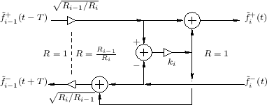
Figure C.23 illustrates a three-multiply
normalized-wave scattering junction [432]. The impedance of
all waveguides (bidirectional delay lines) may be taken to be ![]() .
Scattering junctions may then be implemented as a denormalizing
transformer
.
Scattering junctions may then be implemented as a denormalizing
transformer
![]() , a one-multiply scattering junction
, a one-multiply scattering junction
![]() , and a renormalizing transformer
, and a renormalizing transformer
![]() . Either
transformer may be commuted with the junction and combined with the
other transformer to give a three-multiply normalized-wave scattering
junction. (The transformers are combined on the left in
Fig.C.23).
. Either
transformer may be commuted with the junction and combined with the
other transformer to give a three-multiply normalized-wave scattering
junction. (The transformers are combined on the left in
Fig.C.23).
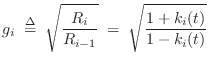
In slightly more detail, a transformer
![]() steps the wave
impedance (left-to-right) from
steps the wave
impedance (left-to-right) from ![]() to
to ![]() . Equivalently, the
normalized force-wave
. Equivalently, the
normalized force-wave
![]() is converted unnormalized form
is converted unnormalized form
![]() . Next there is a physical scattering from impedance
. Next there is a physical scattering from impedance
![]() to
to ![]() (reflection coefficient
(reflection coefficient
![]() ). The outgoing wave to the right is
then normalized by transformer
). The outgoing wave to the right is
then normalized by transformer
![]() to return the wave
impedance back to
to return the wave
impedance back to ![]() for wave propagation within a normalized-wave
delay line to the right. Finally, the right transformer is commuted
left and combined with the left transformer to reduce total
computational complexity to one multiply and three adds.
for wave propagation within a normalized-wave
delay line to the right. Finally, the right transformer is commuted
left and combined with the left transformer to reduce total
computational complexity to one multiply and three adds.
It is important to notice that transformer-normalized junctions may
have a large dynamic range in practice. For example, if
![]() , then Eq.
, then Eq.![]() (C.69) shows that the
transformer coefficients may become as large as
(C.69) shows that the
transformer coefficients may become as large as
![]() . If
. If ![]() is the ``machine epsilon,'' i.e.,
is the ``machine epsilon,'' i.e.,
![]() for typical
for typical ![]() -bit two's complement arithmetic normalized
to lie in
-bit two's complement arithmetic normalized
to lie in ![]() , then the dynamic range of the transformer
coefficients is bounded by
, then the dynamic range of the transformer
coefficients is bounded by
![]() . Thus, while
transformer-normalized junctions trade a multiply for an add, they
require up to
. Thus, while
transformer-normalized junctions trade a multiply for an add, they
require up to ![]() % more bits of dynamic range within the junction
adders. On the other hand, it is very nice to have normalized waves
(unit wave impedance) throughout the digital waveguide network,
thereby limiting the required dynamic range to root physical power in
all propagation paths.
% more bits of dynamic range within the junction
adders. On the other hand, it is very nice to have normalized waves
(unit wave impedance) throughout the digital waveguide network,
thereby limiting the required dynamic range to root physical power in
all propagation paths.
Junction Passivity
In fixed-point implementations, the round-off error and other nonlinear operations should be confined when possible to physically meaningful wave variables. When this is done, it is easy to ensure that signal power is not increased by the nonlinear operations. In other words, nonlinear operations such as rounding can be made passive. Since signal power is proportional to the square of the wave variables, all we need to do is make sure amplitude is never increased by the nonlinearity. In the case of rounding, magnitude truncation, sometimes called ``rounding toward zero,'' is one way to achieve passive rounding. However, magnitude truncation can attenuate the signal excessively in low-precision implementations and in scattering-intensive applications such as the digital waveguide mesh [518]. Another option is error power feedback in which case the cumulative round-off error power averages to zero over time.
A valuable byproduct of passive arithmetic is the suppression of limit cycles and overflow oscillations [432]. Formally, the signal power of a conceptually infinite-precision implementation can be taken as a Lyapunov function bounding the squared amplitude of the finite-precision implementation.
The Kelly-Lochbaum and one-multiply scattering junctions are structurally lossless [500,460] (see also
§C.17) because they have only one parameter ![]() (or
(or
![]() ), and all quantizations of the parameter within the allowed
interval
), and all quantizations of the parameter within the allowed
interval ![]() (or
(or ![]() ) correspond to lossless
scattering.C.6
) correspond to lossless
scattering.C.6
In the Kelly-Lochbaum and one-multiply scattering junctions, because they are structurally lossless, we need only double the number of bits at the output of each multiplier, and add one bit of extended dynamic range at the output of each two-input adder. The final outgoing waves are thereby exactly computed before they are finally rounded to the working precision and/or clipped to the maximum representable magnitude.
For the Kelly-Lochbaum scattering junction, given ![]() -bit signal samples
and
-bit signal samples
and ![]() -bit reflection coefficients, the reflection and transmission
multipliers produce
-bit reflection coefficients, the reflection and transmission
multipliers produce ![]() and
and ![]() bits, respectively, and each of the
two additions adds one more bit. Thus, the intermediate word length
required is
bits, respectively, and each of the
two additions adds one more bit. Thus, the intermediate word length
required is ![]() bits, and this must be rounded without
amplification down to
bits, and this must be rounded without
amplification down to ![]() bits for the final outgoing samples. A similar
analysis gives also that the one-multiply scattering junction needs
bits for the final outgoing samples. A similar
analysis gives also that the one-multiply scattering junction needs ![]() bits for the extended precision intermediate results before final rounding
and/or clipping.
bits for the extended precision intermediate results before final rounding
and/or clipping.
To formally show that magnitude truncation is sufficient to suppress
overflow oscillations and limit cycles in waveguide networks built using
structurally lossless scattering junctions, we can look at the signal power
entering and leaving the junction. A junction is passive if the power
flowing away from it does not exceed the power flowing into it. The total
power flowing away from the ![]() th junction is bounded by the incoming power
if
th junction is bounded by the incoming power
if
![$\displaystyle \underbrace{\frac{[f^{{+}}_i(t)]^2}{R_i(t)}
+ \frac{[f^{{-}}_{i-1...
...t-T)]^2}{R_{i-1}(t)}
+ \frac{[f^{{-}}_i(t)]^2}{R_i(t)}}_{\mbox{incoming power}}$](http://www.dsprelated.com/josimages_new/pasp/img3656.png)
Let
Thus, if the junction computations do not increase either of the output force amplitudes, no signal power is created. An analogous conclusion is reached for velocity scattering junctions.
Unlike the structurally lossless cases, the (four-multiply) normalized
scattering junction has two parameters,
![]() and
and
![]() , and these can ``get out of synch'' in the
presence of quantization. Specifically, let
, and these can ``get out of synch'' in the
presence of quantization. Specifically, let
![]() denote the quantized value of
denote the quantized value of ![]() , and let
, and let
![]() denote the quantized value of
denote the quantized value of ![]() . Then it is no longer the
case in general that
. Then it is no longer the
case in general that
![]() . As a result, the
normalized scattering junction is not structurally lossless in the presence
of coefficient quantization. A few lines of algebra shows that a passive
rounding rule for the normalized junction must depend on the sign of the
wave variable being computed, the sign of the coefficient quantization
error, and the sign of at least one of the two incoming traveling waves.
We can assume one of the coefficients is exact for passivity purposes, so
assume
. As a result, the
normalized scattering junction is not structurally lossless in the presence
of coefficient quantization. A few lines of algebra shows that a passive
rounding rule for the normalized junction must depend on the sign of the
wave variable being computed, the sign of the coefficient quantization
error, and the sign of at least one of the two incoming traveling waves.
We can assume one of the coefficients is exact for passivity purposes, so
assume
![]() and define
and define
![]() , where
, where
![]() denotes largest quantized value less than or equal to
denotes largest quantized value less than or equal to ![]() .
In this case we have
.
In this case we have
![]() . Therefore,
. Therefore,
The three-multiply normalized scattering junction is easier to ``passify.''
While the transformer is not structurally lossless, its simplicity allows
it to be made passive simply by using non-amplifying rounding on both of
its coefficients as well as on its output wave variables. (The transformer
is passive when the product of its coefficients has magnitude less than or
equal to ![]() .) Since there are no additions following the transformer
multiplies, double-precision adders are not needed. However, precision and
a half is needed in the junction adders to accommodate the worst-case
increased dynamic range. Since the one-multiply junction is structurally
lossless, the overall junction is passive if non-amplifying rounding is
applied to
.) Since there are no additions following the transformer
multiplies, double-precision adders are not needed. However, precision and
a half is needed in the junction adders to accommodate the worst-case
increased dynamic range. Since the one-multiply junction is structurally
lossless, the overall junction is passive if non-amplifying rounding is
applied to ![]() ,
, ![]() , and the outgoing wave variables from the
transformer and from the one-multiply junction.
, and the outgoing wave variables from the
transformer and from the one-multiply junction.
In summary, a general means of obtaining passive waveguide junctions is to compute exact results internally, and apply saturation (clipping on overflow) and magnitude truncation (truncation toward zero) to the final outgoing wave variables. Because the Kelly-Lochbaum and one-multiply junctions are structurally lossless, exact intermediate results are obtainable using extended internal precision. For the (four-multiply) normalized scattering junction, a passive rounding rule can be developed based on two sign bits. For the three-multiply normalized scattering junction, it is sufficient to apply magnitude truncation to the transformer coefficients and all outgoing wave variables.
Digital Waveguide Filters
A Digital Waveguide Filter (DWF) can be defined as any digital filter built by stringing together digital waveguides.C.7 In the case of a cascade combination of unit-length waveguide sections, they are essentially the same as microwave filters [372] and unit element filters [136] (Appendix F). This section shows how DWFs constructed as a cascade chain of waveguide sections, and reflectively terminated, can be transformed via elementary manipulations to well known ladder and lattice digital filters, such as those used in speech modeling [297,363].
DWFs may be derived conceptually by sampling the unidirectional traveling waves in a system of ideal, lossless waveguides. Sampling is across time and space. Thus, variables in a DWF structure are equal exactly (at the sampling times and positions, to within numerical precision) to variables propagating in the physical medium in an interconnection of uniform 1D waveguides.
Ladder Waveguide Filters
An important class of DWFs can be constructed as a linear cascade
chain of digital waveguide sections, as shown in Fig.C.24 (a
slightly abstracted version of Fig.C.19). Each block labeled
![]() stands for a state-less Kelly-Lochbaum scattering junction
(§C.8.4) interfacing between wave impedances
stands for a state-less Kelly-Lochbaum scattering junction
(§C.8.4) interfacing between wave impedances ![]() and
and ![]() . We call this a ladder waveguide filter structure.
It is an exact bandlimited discrete-time model of a sequence of wave
impedances
. We call this a ladder waveguide filter structure.
It is an exact bandlimited discrete-time model of a sequence of wave
impedances ![]() , as used in the Kelly-Lochbaum piecewise-cylindrical
acoustic-tube model for the vocal tract in the context of voice
synthesis (Fig.6.2). The delays between scattering
junctions along both the top and bottom signal paths make it possible
to compute all of the scattering junctions in parallel--a property
that is becoming increasingly valuable in signal-processing
architectures.
, as used in the Kelly-Lochbaum piecewise-cylindrical
acoustic-tube model for the vocal tract in the context of voice
synthesis (Fig.6.2). The delays between scattering
junctions along both the top and bottom signal paths make it possible
to compute all of the scattering junctions in parallel--a property
that is becoming increasingly valuable in signal-processing
architectures.
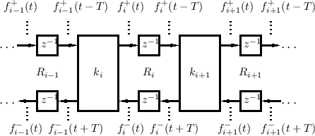
To transform the DWF of Fig.C.24 to a conventional ladder digital filter structure, as used in speech modeling [297,363], we need to (1) terminate on the right with a pure reflection and (2) eliminate the delays along the top signal path. We will do this in stages so as to point out a valuable intermediate case.
Reflectively Terminated Waveguide Filters
A reflecting termination occurs when the wave impedance of the next section is either zero or infinity (§C.8.1). Since Fig.C.24 is labeled for force waves, an infinite terminating impedance on the right results in
Half-Rate Ladder Waveguide Filters
The delays preceding the two inputs to each scattering junction can be ``pushed'' into the junction and then ``pulled'' out to the outputs and combine with the delays there. (This is easy to show using the Kelly-Lochbaum scattering junction derived in §C.8.4.) By performing this operation on every other section in the DWF chain, the half-rate ladder waveguide filter shown in Fig.C.25 is obtained [432].
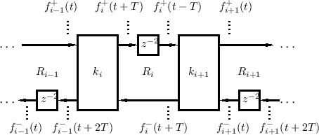
This ``half-rate'' ladder DWF is so-called because its sampling rate can be cut in half due to each delay being two-samples long. It has advantages worth considering, which will become clear after we have derived conventional ladder digital filters below. Note that now pairs of scattering junctions can be computed in parallel, and an exact physical interpretation remains. That is, it can still be used as a general purpose physical modeling building block in this more efficient (half-rate) form.
Note that when the sampling rate is halved, the physical wave
variables (computed by summing two traveling-wave components) are at
the same time only every other spatial sample. In particular, the
physical transverse forces on the right side of scattering junctions
![]() and
and ![]() in Fig.C.25 are
in Fig.C.25 are
![\begin{eqnarray*}
f_i(t+T)&=&f^{{+}}_i(t+T)+f^{{-}}_i(t+T)\\ [5pt]
f_{i+1}(t)&=&f^{{+}}_{i+1}(t)+f^{{-}}_{i+1}(t) \end{eqnarray*}](http://www.dsprelated.com/josimages_new/pasp/img3681.png)
respectively. In the half-rate case, adjacent spatial samples are
separated in time by half a temporal sample ![]() . If physical
variables are needed only for even-numbered (or odd-numbered) spatial
samples, then there is no relative time skew, but more generally,
things like collision detection, such as for slap-bass string-models
(§9.1.6), can be affected. In summary, the half-rate ladder
waveguide filter has an alternating half-sample time skew from section
to section when used as a physical modeling building block.
. If physical
variables are needed only for even-numbered (or odd-numbered) spatial
samples, then there is no relative time skew, but more generally,
things like collision detection, such as for slap-bass string-models
(§9.1.6), can be affected. In summary, the half-rate ladder
waveguide filter has an alternating half-sample time skew from section
to section when used as a physical modeling building block.
Conventional Ladder Filters
Given a reflecting termination on the right, the half-rate DWF chain of Fig.C.25 can be reduced further to the conventional ladder/lattice filter structure shown in Fig.C.26.
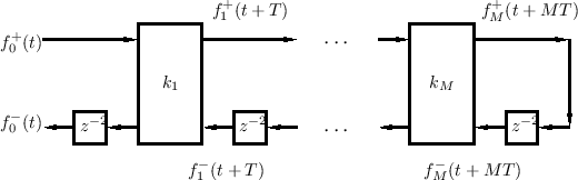
To make a standard ladder/lattice filter, the sampling rate is cut in
half (i.e., replace ![]() by
by ![]() ), and the scattering junctions are
typically implemented in one-multiply form (§C.8.5) or
normalized form (§C.8.6), etc. Conventionally, if the
graph of the scattering junction is nonplanar, as it is for the
one-multiply junction, the filter is called a lattice filter;
it is called a ladder filter when the graph is planar, as it is
for normalized and Kelly-Lochbaum scattering junctions. For all-pole
transfer functions
), and the scattering junctions are
typically implemented in one-multiply form (§C.8.5) or
normalized form (§C.8.6), etc. Conventionally, if the
graph of the scattering junction is nonplanar, as it is for the
one-multiply junction, the filter is called a lattice filter;
it is called a ladder filter when the graph is planar, as it is
for normalized and Kelly-Lochbaum scattering junctions. For all-pole
transfer functions
![]() , the Durbin
recursion can be used to compute the reflection coefficients
, the Durbin
recursion can be used to compute the reflection coefficients ![]() from the desired transfer-function denominator polynomial coefficients
[449]. To implement arbitrary transfer-function zeros, a
linear combination of delay-element outputs is formed using weights
that are called ``tap parameters'' [173,297].
from the desired transfer-function denominator polynomial coefficients
[449]. To implement arbitrary transfer-function zeros, a
linear combination of delay-element outputs is formed using weights
that are called ``tap parameters'' [173,297].
To create Fig.C.26 from Fig.C.24, all delays along the top rail
are pushed to the right until they have all been worked around to the
bottom rail. In the end, each bottom-rail delay becomes ![]() seconds
instead of
seconds
instead of ![]() seconds. Such an operation is possible because of the
termination at the right by an infinite (or zero) wave impedance.
Note that there is a progressive one-sample time advance from section
to section. The time skews for the right-going (or left-going)
traveling waves can be determined simply by considering how many
missing (or extra) delays there are between that signal and the
unshifted signals at the far left.
seconds. Such an operation is possible because of the
termination at the right by an infinite (or zero) wave impedance.
Note that there is a progressive one-sample time advance from section
to section. The time skews for the right-going (or left-going)
traveling waves can be determined simply by considering how many
missing (or extra) delays there are between that signal and the
unshifted signals at the far left.
Due to the reflecting termination, conventional lattice filters cannot
be extended to the right in any physically meaningful way. Also,
creating network topologies more complex than a simple linear cascade
(or acyclic tree) of waveguide sections is not immediately possible
because of the delay-free path along the top rail. In particular, the
output ![]() cannot be fed back to the input
cannot be fed back to the input ![]() . Nevertheless,
as we have derived, there is an exact physical interpretation (with
time skew) for the conventional ladder/lattice digital filter.
. Nevertheless,
as we have derived, there is an exact physical interpretation (with
time skew) for the conventional ladder/lattice digital filter.
Power-Normalized Waveguide Filters
Above, we adopted the convention that the time variation of the wave
impedance did not alter the traveling force waves ![]() . In this
case, the power represented by a traveling force wave is modulated by
the changing wave impedance as it propagates. The signal power
becomes inversely proportional to wave impedance:
. In this
case, the power represented by a traveling force wave is modulated by
the changing wave impedance as it propagates. The signal power
becomes inversely proportional to wave impedance:
![$\displaystyle {\cal I}_i(t,x)
= {\cal I}^{+}_i(t,x)+{\cal I}^{-}_i(t,x)
= \frac{[f^{{+}}_i(t,x)]^2-[f^{{-}}_i(t,x)]^2}{R_i(t)}
$](http://www.dsprelated.com/josimages_new/pasp/img3691.png)
In [432,433], three methods are discussed for making signal power invariant with respect to time-varying branch impedances:
- The normalized waveguide scheme compensates for power
modulation by scaling the signals leaving the delays so as to give
them the same power coming out as they had going in. It requires two
additional scaling multipliers per waveguide junction.
- The normalized wave approach [297] propagates
rms-normalized waves in the waveguide. In this case, each
delay-line contains
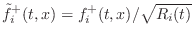 and
and
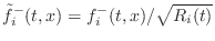 . In this case, the power
stored in the delays does not change when the wave impedance
changes. This is the basis of the normalized ladder filter
(NLF) [174,297]. Unfortunately, four
multiplications are obtained at each scattering junction.
. In this case, the power
stored in the delays does not change when the wave impedance
changes. This is the basis of the normalized ladder filter
(NLF) [174,297]. Unfortunately, four
multiplications are obtained at each scattering junction.
- The transformer-normalized waveguide approach changes the
wave impedance at the output of the delay back to what it was at the
time it entered the delay using a ``transformer'' (defined in
§C.16).
The transformer-normalized DWF junction is shown in Fig.C.27
[432]. As derived in §C.16, the transformer ``turns
ratio'' ![]() is given by
is given by
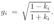
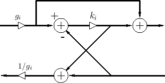 |
So, as in the normalized waveguide case, for the price of two extra multiplies per section, we can implement time-varying digital filters which do not modulate stored signal energy. Moreover, transformers enable the scattering junctions to be varied independently, without having to propagate time-varying impedance ratios throughout the waveguide network.
It can be shown [433] that cascade waveguide chains built using transformer-normalized waveguides are equivalent to those using normalized-wave junctions. Thus, the transformer-normalized DWF in Fig.C.27 and the wave-normalized DWF in Fig.C.22 are equivalent. One simple proof is to start with a transformer (§C.16) and a Kelly-Lochbaum junction (§C.8.4), move the transformer scale factors inside the junction, combine terms, and arrive at Fig.C.22. One practical benefit of this equivalence is that the normalized ladder filter (NLF) can be implemented using only three multiplies and three additions instead of the usual four multiplies and two additions.
The transformer-normalized scattering junction is also the basis of the digital waveguide oscillator (§C.17).
``Traveling Waves'' in Lumped Systems
One of the topics in classical network theory is the reflection and transmission, or scattering formulation for lumped networks [35]. Lumped scattering theory also serves as the starting point for deriving wave digital filters (the subject of Appendix F). In this formulation, forces (voltages) and velocities (currents) are replaced by so-called wave variables
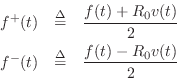
where ![]() is an arbitrary reference impedance.
Since the above wave variables have dimensions of force, they
are specifically force waves. The corresponding velocity
waves are
is an arbitrary reference impedance.
Since the above wave variables have dimensions of force, they
are specifically force waves. The corresponding velocity
waves are
![\begin{eqnarray*}
v^{+}(t) &\isdef & \frac{1}{2}[v(t) + f(t)/R_0], \\
v^{-}(t) &\isdef & \frac{1}{2}[v(t) - f(t)/R_0].
\end{eqnarray*}](http://www.dsprelated.com/josimages_new/pasp/img3698.png)
Dropping the time argument, since it is always `(t)', we see that
and
These are the basic relations for traveling waves in an ideal medium such as an ideal vibrating string or acoustic tube. Using voltage and current gives elementary transmission line theory.
Reflectance of an Impedance
Let ![]() denote the driving-point impedance of an arbitrary
continuous-time LTI system. Then, by definition,
denote the driving-point impedance of an arbitrary
continuous-time LTI system. Then, by definition,
![]() where
where ![]() and
and ![]() denote the Laplace transforms
of the applied force and resulting velocity, respectively.
The wave variable decomposition in Eq.
denote the Laplace transforms
of the applied force and resulting velocity, respectively.
The wave variable decomposition in Eq.![]() (C.74) gives
(C.74) gives
![$\displaystyle R(s) \left[\frac{F^{+}(s) - F^{-}(s)}{R_0}\right]$](http://www.dsprelated.com/josimages_new/pasp/img3712.png)
![$\displaystyle \,\,\Rightarrow\,\,F^{-}(s) \left[\frac{R(s)}{R_0}+1\right]$](http://www.dsprelated.com/josimages_new/pasp/img3713.png)
![$\displaystyle F^{+}(s) \left[\frac{R(s)}{R_0}-1\right]$](http://www.dsprelated.com/josimages_new/pasp/img3714.png)
![$\displaystyle F^{+}(s) \left[\frac{R(s)-R_0}{R(s)+R_0}\right]$](http://www.dsprelated.com/josimages_new/pasp/img3716.png)
We may call
We are working with reflectance for force waves.
Using the elementary relations Eq.![]() (C.73), i.e.,
(C.73), i.e.,
![]() and
and
![]() , we immediately obtain the corresponding
velocity-wave reflectance:
, we immediately obtain the corresponding
velocity-wave reflectance:

Properties of Passive Impedances
It is well known that a real impedance ![]() (in Ohms, for example) is
passive so long as
(in Ohms, for example) is
passive so long as ![]() . A passive impedance cannot
create energy. On the other hand, if
. A passive impedance cannot
create energy. On the other hand, if ![]() , the impedance is
active and has some energy source. The concept of
passivity can be extended to complex frequency-dependent impedances
, the impedance is
active and has some energy source. The concept of
passivity can be extended to complex frequency-dependent impedances
![]() as well: A complex impedance
as well: A complex impedance
![]() is
passive if
is
passive if ![]() is positive real, where
is positive real, where ![]() is the
Laplace-transform variable. The positive-real property is discussed in
§C.11.2 below.
is the
Laplace-transform variable. The positive-real property is discussed in
§C.11.2 below.
This section explores some implications of the positive real condition for passive impedances. Specifically, §C.11.1 considers the nature of waves reflecting from a passive impedance in general, looking at the reflection transfer function, or reflectance, of a passive impedance. To provide further details, Section C.11.2 derives some mathematical properties of positive real functions, particularly for the discrete-time case. Application examples appear in §9.2.1 and §9.2.1.
Passive Reflectances
From Eq.![]() (C.75),
we have that the reflectance seen at a continuous-time impedance
(C.75),
we have that the reflectance seen at a continuous-time impedance
![]() is given for force waves by
is given for force waves by
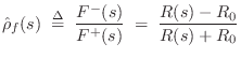
where
In particular,
If the impedance ![]() goes to infinity (becomes rigid), then
goes to infinity (becomes rigid), then
![]() approaches
approaches ![]() , a result which agrees with an analysis of
rigid string terminations (p.
, a result which agrees with an analysis of
rigid string terminations (p. ![]() ). Similarly, when the
impedance goes to zero,
). Similarly, when the
impedance goes to zero,
![]() becomes
becomes ![]() , which agrees with
the physics of a string with a free end. In acoustic stringed
instruments, bridges are typically quite rigid, so that
, which agrees with
the physics of a string with a free end. In acoustic stringed
instruments, bridges are typically quite rigid, so that
![]() for all
for all ![]() . If a body resonance is
strongly coupled through the bridge,
. If a body resonance is
strongly coupled through the bridge,
![]() can be
significantly smaller than 1 at the resonant frequency
can be
significantly smaller than 1 at the resonant frequency ![]() .
.
Solving for ![]() in Eq.
in Eq.![]() (C.77), we can characterize every
impedance in terms of its reflectance:
(C.77), we can characterize every
impedance in terms of its reflectance:
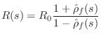
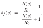
In the discrete-time case, which may be related to the continuous-time
case by the bilinear transform (§7.3.2), we have the same basic
relations, but in the ![]() plane:
plane:


where
Mathematically, any stable transfer function having these properties may be called a Schur function. Thus, the discrete-time reflectance
Note that Eq.![]() (C.79) may be obtained from the general formula for
scattering at a loaded waveguide junction for the case of a single
waveguide (
(C.79) may be obtained from the general formula for
scattering at a loaded waveguide junction for the case of a single
waveguide (![]() ) terminated by a lumped load (§C.12).
) terminated by a lumped load (§C.12).
In the limit as damping goes to zero (all poles of ![]() converge to
the unit circle),
the reflectance
converge to
the unit circle),
the reflectance
![]() becomes a digital allpass filter. Similarly,
becomes a digital allpass filter. Similarly,
![]() becomes a continuous-time allpass filter as the poles of
becomes a continuous-time allpass filter as the poles of
![]() approach the
approach the ![]() axis.
axis.
Recalling that a lossless impedance is called a reactance
(§7.1), we can say that every reactance gives rise to an
allpass reflectance. Thus, for example, waves reflecting off a
mass at the end of a vibrating string will be allpass filtered,
because the driving-point impedance of a mass (![]() ) is a pure
reactance. In particular, the force-wave reflectance of a mass
) is a pure
reactance. In particular, the force-wave reflectance of a mass ![]() terminating an ideal string having wave impedance
terminating an ideal string having wave impedance ![]() is
is
![]() , which is a continuous-time allpass filter having
a pole at
, which is a continuous-time allpass filter having
a pole at ![]() and a zero at
and a zero at ![]() .
.
It is intuitively reasonable that a passive reflection gain cannot
exceed ![]() at any frequency (i.e., the reflectance is a Schur filter,
as defined in Eq.
at any frequency (i.e., the reflectance is a Schur filter,
as defined in Eq.![]() (C.79)). It is also reasonable that lossless
reflection would have a gain of 1 (i.e., it is allpass).
(C.79)). It is also reasonable that lossless
reflection would have a gain of 1 (i.e., it is allpass).
Note that reflection filters always have an equal number of poles and
zeros, as can be seen from Eq.![]() (C.76) above. This property is
preserved by the bilinear transform, so it holds in both the
continuous- and discrete-time cases.
(C.76) above. This property is
preserved by the bilinear transform, so it holds in both the
continuous- and discrete-time cases.
Reflectance and Transmittance of a Yielding String Termination
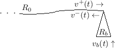
Consider the special case of a reflection and transmission at a
yielding termination, or ``bridge'', of an ideal vibrating
string on its right end, as shown in Fig.C.28. Denote the
incident and reflected velocity waves by ![]() and
and ![]() ,
respectively, and similarly denote the force-wave components by
,
respectively, and similarly denote the force-wave components by
![]() and
and
![]() . Finally, denote the velocity of the
termination itself by
. Finally, denote the velocity of the
termination itself by
![]() , and its force-wave
reflectance by
, and its force-wave
reflectance by

The bridge velocity is given by
![$\displaystyle \hat{\tau}_f(s) \isdefs \frac{F_b(s)}{F^{+}(s)}
\eqsp \frac{R_0[V^{+}(s)-V^{-}(s)]}{R_0V^{+}(s)}
\eqsp 1+\hat{\rho}_f(s)
$](http://www.dsprelated.com/josimages_new/pasp/img3757.png)
Power-Complementary Reflection and Transmission
We can show that the reflectance and transmittance of the yielding termination are power complementary. That is, the reflected and transmitted signal-power sum to yield the incident signal-power.
The average power incident at the bridge at frequency ![]() can be
expressed in the frequency domain as
can be
expressed in the frequency domain as
![]() .
The reflected power is then
.
The reflected power is then
![]() . Removing the minus sign, which can be
associated with reversed direction of travel, we obtain that the
power reflection frequency response is
. Removing the minus sign, which can be
associated with reversed direction of travel, we obtain that the
power reflection frequency response is
![]() , which
generalizes by analytic continuation to
, which
generalizes by analytic continuation to
![]() . The power
transmittance is given by
. The power
transmittance is given by
Positive Real Functions
Any passive driving-point impedance, such as the impedance of a
violin bridge, is positive real. Positive real functions have
been studied extensively in the continuous-time case in the context of
network synthesis [68,524]. Very little, however, seems
to be available in the discrete time case. This section (reprinted
from [428]) summarizes the main properties of positive real
function in the ![]() plane (i.e., the discrete-time case).
plane (i.e., the discrete-time case).
Definition.
A complex valued function of a complex variable ![]() is said to be
positive real (PR) if
is said to be
positive real (PR) if
We now specialize to the subset of functions ![]() representable as a
ratio of finite-order polynomials in
representable as a
ratio of finite-order polynomials in ![]() . This class of ``rational''
functions is the set of all transfer functions of finite-order
time-invariant linear systems, and we write
. This class of ``rational''
functions is the set of all transfer functions of finite-order
time-invariant linear systems, and we write ![]() to denote a member
of this class. We use the convention that stable, minimum phase
systems are analytic and nonzero in the strict outer
disk.C.8 Condition (1) implies
that for
to denote a member
of this class. We use the convention that stable, minimum phase
systems are analytic and nonzero in the strict outer
disk.C.8 Condition (1) implies
that for ![]() to be PR, the polynomial coefficients must be real,
and therefore complex poles and zeros must exist in conjugate
pairs. We assume from this point on that
to be PR, the polynomial coefficients must be real,
and therefore complex poles and zeros must exist in conjugate
pairs. We assume from this point on that
![]() satisfies (1).
From (2) we derive the facts below.
satisfies (1).
From (2) we derive the facts below.
Property 1. A real rational function ![]() is PR iff
is PR iff
![]() .
.
Proof. Expressing ![]() in polar form gives
in polar form gives
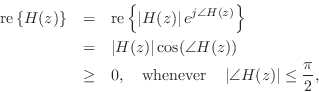
since the zeros of ![]() are isolated.
are isolated.
![]()
Property 2. ![]() is PR iff
is PR iff ![]() is PR.
is PR.
Proof. Assuming ![]() is PR, we have by Property 1,
is PR, we have by Property 1,
Property 3. A PR function ![]() is analytic and nonzero in
the strict outer disk.
is analytic and nonzero in
the strict outer disk.
Proof. (By contradiction)
Without loss of generality, we treat only ![]() order polynomials
order polynomials
The general (normalized) causal, finite-order, linear,
time-invariant transfer function may be written

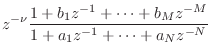
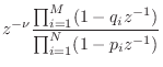

where
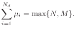
Suppose there is a pole of multiplicity ![]() outside the unit circle.
Without loss of generality, we may set
outside the unit circle.
Without loss of generality, we may set ![]() , and
, and
![]() with
with ![]() . Then for
. Then for ![]() near
near ![]() , we have
, we have
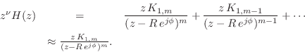
Consider the circular neighborhood of radius ![]() described by
described by
![]() . Since
. Since ![]() we may
choose
we may
choose
![]() so that all points
so that all points ![]() in this neighborhood lie
outside the unit circle. If we write the residue of the factor
in this neighborhood lie
outside the unit circle. If we write the residue of the factor
![]() in polar form as
in polar form as
![]() , then we have,
for sufficiently small
, then we have,
for sufficiently small ![]() ,
,
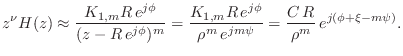
Therefore, approaching the pole
Corollary. In equation Eq.![]() (C.80),
(C.80), ![]() .
.
Proof. If ![]() , then there are
, then there are ![]() poles at
infinity. As
poles at
infinity. As
![]() ,
,
![]() , we must have
, we must have ![]() .
.
![]()
Corollary. The log-magnitude of a PR function has zero mean on the unit circle.
This is a general property of stable, minimum-phase transfer functions which follows immediately from the argument principle [297,326].
Corollary. A rational PR function has an equal number of poles and zeros all of which are in the unit disk.
This really a convention for numbering poles and zeros. In Eq.![]() (C.80),
we have
(C.80),
we have ![]() , and all poles and zeros inside the unit disk. Now, if
, and all poles and zeros inside the unit disk. Now, if
![]() then we have
then we have ![]() extra poles at
extra poles at ![]() induced by the numerator.
If
induced by the numerator.
If ![]() , then
, then ![]() zeros at the origin appear from the denominator.
zeros at the origin appear from the denominator.
Corollary. Every pole on the unit circle of a positive real function must be simple with a real and positive residue.
Proof.
We repeat the previous argument using a semicircular neighborhood of
radius ![]() about the point
about the point
![]() to obtain
to obtain
In order to have
Corollary.
If ![]() is PR with a zero at
is PR with a zero at
![]() , then
, then
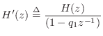
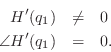
Proof. We may repeat the above for ![]() .
.
Property. Every PR function ![]() has a causal inverse z transform
has a causal inverse z transform ![]() .
.
Proof. This follows immediately from analyticity in the outer disk
[342, pp. 30-36]
However, we may give a more concrete proof as follows.
Suppose ![]() is non-causal. Then there exists
is non-causal. Then there exists
![]() such that
such that
![]() .
We have,
.
We have,

Hence, ![]() has at least one pole at infinity and cannot be PR by Property 3.
Note that this pole at infinity cannot be cancelled since otherwise
has at least one pole at infinity and cannot be PR by Property 3.
Note that this pole at infinity cannot be cancelled since otherwise
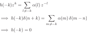
which contradicts the hypothesis that ![]() is non-causal.
is non-causal.
![]()
Property.
![]() is PR iff it is analytic for
is PR iff it is analytic for
![]() , poles on the
unit circle are simple with real and positive residues, and
re
, poles on the
unit circle are simple with real and positive residues, and
re![]() for
for
![]() .
.
Proof. If ![]() is positive real, the conditions stated hold by virtue
of Property 3 and the definition of positive real.
is positive real, the conditions stated hold by virtue
of Property 3 and the definition of positive real.
To prove the converse, we first show nonnegativity on the upper semicircle implies nonnegativity over the entire circle.
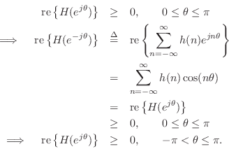
Alternatively, we might simply state that
![]() real implies
re
real implies
re![]() is even in
is even in ![]() .
.
Next, since the function ![]() is analytic everywhere except at
is analytic everywhere except at
![]() , it follows that
, it follows that
![]() is analytic wherever
is analytic wherever
![]() is finite. There are no poles of
is finite. There are no poles of ![]() outside the unit
circle due to the analyticity assumption, and poles on the unit circle
have real and positive residues. Referring again to the limiting form
Eq.
outside the unit
circle due to the analyticity assumption, and poles on the unit circle
have real and positive residues. Referring again to the limiting form
Eq.![]() (C.81) of
(C.81) of ![]() near a pole on the unit circle at
near a pole on the unit circle at ![]() ,
we see that, as
,
we see that, as
![]() , we have
, we have
since the residue
For example, if a transfer function is known to be asymptotically stable, then a frequency response with nonnegative real part implies that the transfer function is positive real.
Note that consideration of ![]() leads to analogous necessary and sufficient
conditions for
leads to analogous necessary and sufficient
conditions for ![]() to be positive real in terms of its
zeros instead of poles.
to be positive real in terms of its
zeros instead of poles.
![]()
Relation to Stochastic Processes
Property.
If a stationary random process ![]() has a rational power spectral
density
has a rational power spectral
density
![]() corresponding to an autocorrelation function
corresponding to an autocorrelation function
![]() , then
, then
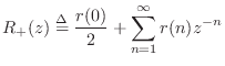
Proof.
By the representation theorem [19, pp. 98-103] there exists
an asymptotically stable filter
![]() which will produce a
realization of
which will produce a
realization of ![]() when driven by white noise, and we have
when driven by white noise, and we have
![]() . We define the analytic continuation
of
. We define the analytic continuation
of
![]() by
by
![]() . Decomposing
. Decomposing ![]() into a sum of
causal and anti-causal components gives
into a sum of
causal and anti-causal components gives

where ![]() is found by equating coefficients of like powers of
is found by equating coefficients of like powers of ![]() in
in
Since the poles of ![]() and
and ![]() are the same,
it only remains to be shown that
re
are the same,
it only remains to be shown that
re![]() .
.
Since spectral power is nonnegative,
![]() for all
for all ![]() , and so
, and so
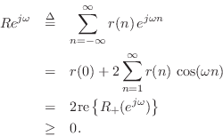
![]()
Relation to Schur Functions
Definition. A Schur function ![]() is defined as a complex function analytic and of modulus not exceeding
unity in
is defined as a complex function analytic and of modulus not exceeding
unity in ![]() .
.
Property. The function
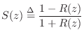
is a Schur function if and only if
Proof.
Suppose ![]() is positive real. Then for
is positive real. Then for ![]() ,
re
,
re![]() re
re![]() is PR. Consequently,
is PR. Consequently, ![]() is minimum phase which implies all roots of
is minimum phase which implies all roots of ![]() lie in the unit circle.
Thus
lie in the unit circle.
Thus ![]() is analytic in
is analytic in ![]() . Also,
. Also,
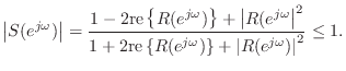
Conversely, suppose ![]() is Schur. Solving Eq.
is Schur. Solving Eq.![]() (C.84) for
(C.84) for ![]() and taking the real part on the unit circle yields
and taking the real part on the unit circle yields
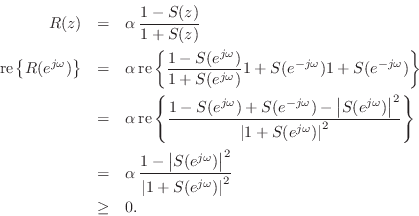
If
![]() is constant, then
is constant, then
![]() is PR. If
is PR. If ![]() is not
constant, then by the maximum principle,
is not
constant, then by the maximum principle, ![]() for
for ![]() . By
Rouche's theorem applied on a circle of radius
. By
Rouche's theorem applied on a circle of radius
![]() ,
,
![]() , on
which
, on
which ![]() , the function
, the function ![]() has the same number of
zeros as the function
has the same number of
zeros as the function ![]() in
in
![]() . Hence,
. Hence, ![]() is
minimum phase which implies
is
minimum phase which implies ![]() is analytic for
is analytic for ![]() . Thus
. Thus
![]() is PR.
is PR.![]()
Relation to functions positive real in the right-half plane
Property.
re![]() for
for
![]() whenever
whenever
Proof.
We shall show that the change of variable
![]() ,
provides a conformal map from the z-plane to the s-plane that takes the
region
,
provides a conformal map from the z-plane to the s-plane that takes the
region
![]() to the region
re
to the region
re![]() . The general formula for a
bilinear conformal mapping of functions of a complex variable is given by
. The general formula for a
bilinear conformal mapping of functions of a complex variable is given by
In general, a bilinear transformation maps circles and lines into circles
and lines [83]. We see that the choice of three specific points
and their images determines the mapping for all ![]() and
and ![]() .
We must have that the imaginary axis in the s-plane maps to the unit circle
in the z-plane.
That is, we may determine the mapping by three points of the form
.
We must have that the imaginary axis in the s-plane maps to the unit circle
in the z-plane.
That is, we may determine the mapping by three points of the form
![]() and
and
![]() .
If we predispose one such mapping by choosing the pairs
.
If we predispose one such mapping by choosing the pairs
![]() and
and
![]() , then we are left with
transformations of the form
, then we are left with
transformations of the form
Letting
There is a bonus associated with the restriction that ![]() be real which
is that
be real which
is that
We have therefore proven
Property.
 PR
PR
The class of mappings of the form Eq.![]() (C.85) which take the exterior of
the unit circle to the right-half plane is larger than the class
Eq.
(C.85) which take the exterior of
the unit circle to the right-half plane is larger than the class
Eq.![]() (C.86). For example, we may precede the transformation
Eq.
(C.86). For example, we may precede the transformation
Eq.![]() (C.86) by any
conformal map which takes the unit disk to the unit disk, and these
mappings have the algebraic form of a first order complex allpass
whose zero lies inside the unit circle.
(C.86) by any
conformal map which takes the unit disk to the unit disk, and these
mappings have the algebraic form of a first order complex allpass
whose zero lies inside the unit circle.
where
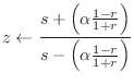
Riemann's theorem may be used to show that Eq.
The bilinear transform is one which is used to map analog filters into
digital filters. Another such mapping is called the matched ![]() transform [362]. It also preserves the positive real
property.
transform [362]. It also preserves the positive real
property.
Property. ![]() is PR if
is PR if ![]() is positive real in the analog
sense, where
is positive real in the analog
sense, where ![]() is interpreted as the sampling period.
is interpreted as the sampling period.
Proof. The mapping
![]() takes the right-half
takes the right-half ![]() -plane to
the outer disk in the
-plane to
the outer disk in the ![]() -plane. Also
-plane. Also ![]() is real if
is real if ![]() is
real. Hence
is
real. Hence ![]() PR implies
PR implies ![]() PR. (Note, however, that
rational functions do not in general map to rational
functions.)
PR. (Note, however, that
rational functions do not in general map to rational
functions.)![]()
These transformations allow application of the large battery of tests which exist for functions positive real in the right-half plane [524].
Special cases and examples
- The sum of positive real functions is positive real.
- The difference of positive real functions is conditionally positive real.
- The product or division of positive real functions is conditionally PR.
 PR
PR
 not PR for
 .
.
Minimum Phase (MP) polynomials in 
All properties of MP polynomials apply without modification to marginally stable allpole transfer functions (cf. Property 2):
- Every first-order MP polynomial is positive real.
- Every first-order MP polynomial
 is such that
 is positive real.
- A PR second-order MP polynomial with complex-conjugate zeros,
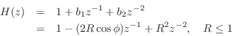
satisfies
If
 , then
re
, then
re has a double zero at
- All polynomials of the form
are positive real. (These have zeros uniformly distributed on a circle of radius
 .)
.)
Miscellaneous Properties
- If all poles and zeros of a PR function are on the unit circle,
then they alternate along the circle. Since this property is
preserved by the bilinear transform, it is true in both the
 and planes. It can be viewed as a consequence of the
 phase bounds for positive-real functions.
- If
 is PR, then so is
 ,
where the prime denotes differentiation in .
,
where the prime denotes differentiation in .
Loaded Waveguide Junctions
In this section, scattering relations will be derived for the general
case of N waveguides meeting at a load. When a load is
present, the scattering is no longer lossless, unless the load itself
is lossless. (i.e., its impedance has a zero real part). For ![]() ,
,
![]() will denote a velocity wave traveling into the junction,
and will be called an ``incoming'' velocity wave as opposed to
``right-going.''C.9
will denote a velocity wave traveling into the junction,
and will be called an ``incoming'' velocity wave as opposed to
``right-going.''C.9
![\includegraphics[width=\twidth]{eps/fNstrings}](http://www.dsprelated.com/josimages_new/pasp/img3925.png) |
Consider first the series junction of ![]() waveguides
containing transverse force and velocity waves. At a series junction,
there is a common velocity while the forces sum. For definiteness, we
may think of
waveguides
containing transverse force and velocity waves. At a series junction,
there is a common velocity while the forces sum. For definiteness, we
may think of ![]() ideal strings intersecting at a single point, and the
intersection point can be attached to a lumped load impedance
ideal strings intersecting at a single point, and the
intersection point can be attached to a lumped load impedance
![]() , as depicted in Fig.C.29 for
, as depicted in Fig.C.29 for ![]() . The presence of
the lumped load means we need to look at the wave variables in the
frequency domain, i.e.,
. The presence of
the lumped load means we need to look at the wave variables in the
frequency domain, i.e.,
![]() for velocity waves and
for velocity waves and
![]() for force waves, where
for force waves, where
![]() denotes
the Laplace transform. In the discrete-time case, we use the
denotes
the Laplace transform. In the discrete-time case, we use the ![]() transform instead, but otherwise the story is identical. The physical
constraints at the junction are
transform instead, but otherwise the story is identical. The physical
constraints at the junction are
| (C.90) | |||
| (C.91) |
where the reference direction for the load force
The parallel junction is characterized by
| (C.92) | |||
| (C.93) |
For example,
The scattering relations for the series junction are derived as
follows, dropping the common argument `![]() ' for simplicity:
' for simplicity:
 |
(C.94) | ||
 |
(C.95) | ||
 |
(C.96) |
where
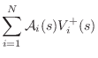
(written to be valid also in the multivariable case involving square impedance matrices
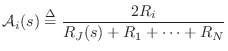
Finally, from the basic relation
Similarly, the scattering relations for the loaded parallel junction
are given by
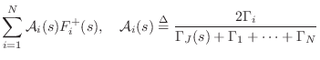
where
It is interesting to note that the junction load is equivalent to an
![]() st waveguide having a (generalized) wave impedance given by the
load impedance. This makes sense when one recalls that a transmission
line can be ``perfectly terminated'' (i.e., suppressing all
reflections from the termination) using a lumped resistor equal in
value to the wave impedance of the transmission line. Thus, as far as
a traveling wave is concerned, there is no difference between a wave
impedance and a lumped impedance of the same value.
st waveguide having a (generalized) wave impedance given by the
load impedance. This makes sense when one recalls that a transmission
line can be ``perfectly terminated'' (i.e., suppressing all
reflections from the termination) using a lumped resistor equal in
value to the wave impedance of the transmission line. Thus, as far as
a traveling wave is concerned, there is no difference between a wave
impedance and a lumped impedance of the same value.
In the unloaded case, ![]() , and we can return to the time
domain and define (for the series junction)
, and we can return to the time
domain and define (for the series junction)
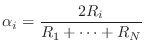
These we call the alpha parameters, and they are analogous to those used to characterize ``adaptors'' in wave digital filters (§F.2.2). For unloaded junctions, the alpha parameters obey
| (C.103) |
and
 |
(C.104) |
In the unloaded case, the series junction scattering relations are given (in
the time domain) by

The alpha parameters provide an interesting and useful parametrization of waveguide junctions. They are explicitly the coefficients of the incoming traveling waves needed to compute junction velocity for a series junction (or junction force or pressure at a parallel junction), and losslessness is assured provided only that the alpha parameters be nonnegative and sum to
Note that in the lossless, equal-impedance case, in which all waveguide
impedances have the same value ![]() , (C.102) reduces to
, (C.102) reduces to
When, furthermore,
An elaborated discussion of ![]() strings intersection at a load is
given in in §9.2.1. Further discussion of the digital waveguide
mesh appears in §C.14.
strings intersection at a load is
given in in §9.2.1. Further discussion of the digital waveguide
mesh appears in §C.14.
Two Coupled Strings
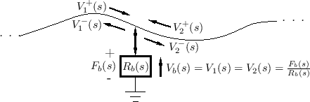
Two Ideal Strings Coupled at an Impedance
A diagram for the two-string case is shown in
Fig. C.30. This situation is a special case of the
loaded waveguide junction, Eq.![]() (C.98), with the
number of waveguides being
(C.98), with the
number of waveguides being ![]() , and the junction load being the
transverse driving-point impedance
, and the junction load being the
transverse driving-point impedance ![]() where the string drives
the bridge. If the bridge is passive, then its impedance
where the string drives
the bridge. If the bridge is passive, then its impedance ![]() is
a positive real function (see §C.11.2). For a direct derivation,
we need only observe that (1) the string velocities of each string
endpoint must each be equal to the velocity of the bridge, or
is
a positive real function (see §C.11.2). For a direct derivation,
we need only observe that (1) the string velocities of each string
endpoint must each be equal to the velocity of the bridge, or
![]() , and (2) the sum of forces of both strings equals the force
applied to the bridge:
, and (2) the sum of forces of both strings equals the force
applied to the bridge:
![]() . The bridge impedance
relates the force and velocity of the bridge via
. The bridge impedance
relates the force and velocity of the bridge via
![]() . Expanding into traveling wave components in the Laplace
domain, we have
. Expanding into traveling wave components in the Laplace
domain, we have
| (C.108) | |||
| (C.109) | |||
| (C.110) | |||
| (C.111) |
or
Given the filter output ![]() , the outgoing traveling velocity waves are
given by
, the outgoing traveling velocity waves are
given by
| (C.112) | |||
| (C.113) |
Thus, the incoming waves are subtracted from the bridge velocity to get the outgoing waves.
Since
![]() when
when
![]() , and vice versa exchanging strings
, and vice versa exchanging strings ![]() and
and ![]() ,
, ![]() may be
interpreted as the transmission admittance filter associated with
the bridge coupling. It can also be interpreted as the bridge admittance
transfer function from every string, since its output is the bridge
velocity resulting from the sum of incident traveling force waves.
may be
interpreted as the transmission admittance filter associated with
the bridge coupling. It can also be interpreted as the bridge admittance
transfer function from every string, since its output is the bridge
velocity resulting from the sum of incident traveling force waves.
A general coupling matrix contains a filter transfer function in each
entry of the matrix. For ![]() strings, each conveying a single type of
wave (e.g., horizontally polarized), the general linear coupling
matrix would have
strings, each conveying a single type of
wave (e.g., horizontally polarized), the general linear coupling
matrix would have ![]() transfer-function entries. In the present
formulation, only one transmission filter is needed, and it is shared
by all the strings meeting at the bridge. It is easy to show that the
shared transmission filter for two coupled strings generalizes to
transfer-function entries. In the present
formulation, only one transmission filter is needed, and it is shared
by all the strings meeting at the bridge. It is easy to show that the
shared transmission filter for two coupled strings generalizes to ![]() strings coupled at a common bridge impedance: From
(C.98), we have
strings coupled at a common bridge impedance: From
(C.98), we have
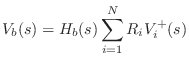
The above sequence of operations is formally similar to the one multiply scattering junction frequently used in digital lattice filters [297]. In this context, it would be better termed the ``one-filter scattering termination.''
When the two strings are identical (as would be appropriate in a model for coupled piano strings), the computation of bridge velocity simplifies to
where

Note that a yielding bridge introduces losses into all attached
strings. Therefore, in a maximally simplified implementation, all
string loop filters (labeled
LPF![]() and
LPF
and
LPF![]() in
Fig.C.31) may be eliminated, resulting in only one
filter--the transmission filter--serving to provide all losses in a
coupled-string simulation. If that transmission filter has no
multiplies, then neither does the entire multi-string simulation.
in
Fig.C.31) may be eliminated, resulting in only one
filter--the transmission filter--serving to provide all losses in a
coupled-string simulation. If that transmission filter has no
multiplies, then neither does the entire multi-string simulation.
Coupled Strings Eigenanalysis
In §6.12.2, general coupling of horizontal and vertical planes of vibration in an ideal string was considered. This eigenanalysis will now be applied here to obtain formulas for the damping and mode tuning caused by the coupling of two identical strings at a bridge. This is the case that arises in pianos [543].
The general formula for linear, time-invariant coupling of two strings can be written, in the frequency domain, as
![$\displaystyle \left[\begin{array}{c} V_1^-(s) \\ [2pt] V_2^-(s) \end{array}\rig...
... \left[\begin{array}{c} V_1^+(s) \\ [2pt] V_2^+(s) \end{array}\right]. \protect$](http://www.dsprelated.com/josimages_new/pasp/img3999.png)
Filling in the elements of this coupling matrix
![$\displaystyle \mathbf{H}_c(s) = \left[\begin{array}{cc} 1-H_b(s) & -H_b(s) \\ [2pt] -H_b(s) & 1-H_b(s) \end{array}\right]
$](http://www.dsprelated.com/josimages_new/pasp/img4001.png)
![$\displaystyle \underline{e}_1 = \left[\begin{array}{c} 1 \\ [2pt] 1 \end{array}...
...uad
\underline{e}_2 = \left[\begin{array}{c} 1 \\ [2pt] -1 \end{array}\right],
$](http://www.dsprelated.com/josimages_new/pasp/img4005.png)
We conclude that ``in-phase vibrations'' see a longer effective string length, lengthened by the phase delay of
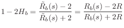
We similarly conclude that the ``anti-phase vibrations'' see no length correction at all, because the bridge point does not move at all in this case. In other words, any bridge termination at a point is rigid with respect to anti-phase vibration of the two strings connected to that point.
The above analysis predicts that, in ``stiffness controlled'' frequency intervals (in which the bridge ``looks like a damped spring''), the ``initial fast decay'' of a piano note should be a measurably flatter than the ``aftersound'' which should be exactly in tune as if the termination were rigid.
Digital Waveguide Mesh
In §C.12, the theory of multiport scattering was derived, i.e.,
the reflections and transmissions that occur when ![]() digital
waveguides having wave impedances
digital
waveguides having wave impedances ![]() are connected together. It
was noted that when
are connected together. It
was noted that when ![]() is a power of two, there are
no multiplies in the scattering relations Eq.
is a power of two, there are
no multiplies in the scattering relations Eq.![]() (C.105), and that
this fact has been used to build multiply-free reverberators and other
structures using digital waveguide meshes
[430,518,146,396,520,521,398,399,401,55,202,321,320,322,422,33].
(C.105), and that
this fact has been used to build multiply-free reverberators and other
structures using digital waveguide meshes
[430,518,146,396,520,521,398,399,401,55,202,321,320,322,422,33].
The Rectilinear 2D Mesh
![\includegraphics[width=4in]{eps/SchematicWaveguideMesh}](http://www.dsprelated.com/josimages_new/pasp/img4008.png)
Figure C.32 shows the basic layout of the rectilinear 2D waveguide mesh. It can be thought of as simulating a plane using 1D digital waveguides in the same way that a tennis racket acts as a membrane composed of 1D strings.
At each node (string intersection), we have the following simple formula for the
node velocity ![]() in terms of the four incoming traveling-wave components:
in terms of the four incoming traveling-wave components:
Dispersion
Since the digital waveguide mesh is lossless by construction (when modeling lossless membranes and volumes), and since it is also linear and time-invariant by construction, being made of ordinary digital filtering computations, there is only one type of error exhibited by the mesh: dispersion. Dispersion can be quantified as an error in propagation speed as a function of frequency and direction along the mesh. The mesh geometry (rectilinear, triangular, hexagonal, tetrahedral, etc.) strongly influences the dispersion properties. Many cases are analyzed in [55] using von Neumann analysis (see also Appendix D).
The triangular waveguide mesh [146] turns out to be the simplest mesh geometry in 2D having the least dispersion variation as a function of direction of propagation on the mesh. In other terms, the triangular mesh is closer to isotropic than all other known elementary geometries. The interpolated waveguide mesh [398] can also be configured to optimize isotropy, but at a somewhat higher compuational cost.
Recent Developments
An interesting approach to dispersion compensation is based on frequency-warping the signals going into the mesh [399]. Frequency warping can be used to compensate frequency-dependent dispersion, but it does not address angle-dependent dispersion. Therefore, frequency-warping is used in conjunction with an isotropic mesh.
The 3D waveguide mesh [518,521,399] is seeing more use for efficient simulation of acoustic spaces [396,182]. It has also been applied to statistical modeling of violin body resonators in [203,202,422,428], in which the digital waveguide mesh was used to efficiently model only the ``reverberant'' aspects of a violin body's impulse response in statistically matched fashion (but close to perceptually equivalent). The ``instantaneous'' filtering by the violin body is therefore modeled using a separate equalizer capturing the important low-frequency body and air modes explicitly. A unified view of the digital waveguide mesh and wave digital filters (§F.1) as particular classes of energy invariant finite difference schemes (Appendix D) appears in [54]. The problem of modeling diffusion at a mesh boundary was addressed in [268], and maximally diffusing boundaries, using quadratic residue sequences, was investigated in [279]; an introduction to this topic is given in §C.14.6 below.
2D Mesh and the Wave Equation
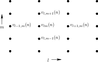
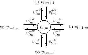 |
Consider the 2D rectilinear mesh, with nodes at positions ![]() and
and
![]() , where
, where ![]() and
and ![]() are integers, and
are integers, and ![]() and
and ![]() denote the
spatial sampling intervals along
denote the
spatial sampling intervals along ![]() and
and ![]() , respectively
(see Fig.C.33).
Then from
Eq.
, respectively
(see Fig.C.33).
Then from
Eq.![]() (C.105) the junction velocity
(C.105) the junction velocity ![]() at time
at time ![]() is given
by
is given
by
These incoming traveling-wave components arrive from the four
neighboring nodes after a one-sample propagation delay. For example,
![]() , arriving from the north, departed from node
, arriving from the north, departed from node
![]() at time
at time ![]() , as
, as
![]() .
Furthermore, the outgoing components at time
.
Furthermore, the outgoing components at time
![]() will arrive at the neighboring nodes
one sample in the future at time
will arrive at the neighboring nodes
one sample in the future at time ![]() .
For example,
.
For example,
![]() will become
will become
![]() .
Using these relations, we can
write
.
Using these relations, we can
write
![]() in terms of the four outgoing waves from its
neighbors at time
in terms of the four outgoing waves from its
neighbors at time ![]() :
:
where, for instance,
This may be shown in detail by writing
![\begin{eqnarray*}
v_{lm}(n-1)
&=& \frac{1}{2}[v_{lm}^{+\textsc{n}}(n-1) + \cdot...
...}^{-\textsc{n}}(n-1) + \cdots + v_{lm}^{-\textsc{w}}(n-1)\right]
\end{eqnarray*}](http://www.dsprelated.com/josimages_new/pasp/img4027.png)
so that
![\begin{eqnarray*}
v_{lm}(n-1)
&=& \frac{1}{2}[v_{lm}^{-\textsc{n}}(n-1) + \cdot...
...
v_{l,m-1}^{+\textsc{n}}(n) +
v_{l-1,m}^{+\textsc{e}}(n)\right].
\end{eqnarray*}](http://www.dsprelated.com/josimages_new/pasp/img4028.png)
Adding Equations (C.116-C.116), replacing
terms such as
![]() with
with
![]() , yields a computation in terms of physical node velocities:
, yields a computation in terms of physical node velocities:
![\begin{eqnarray*}
\lefteqn{v_{lm}(n+1) + v_{lm}(n-1) = } \\
& & \frac{1}{2}\left[
v_{l,m+1}(n) +
v_{l+1,m}(n) +
v_{l,m-1}(n) +
v_{l-1,m}(n)\right]
\end{eqnarray*}](http://www.dsprelated.com/josimages_new/pasp/img4031.png)
Thus, the rectangular waveguide mesh satisfies this equation
giving a formula for the velocity at node ![]() , in terms of
the velocity at its neighboring nodes one sample earlier, and itself
two samples earlier. Subtracting
, in terms of
the velocity at its neighboring nodes one sample earlier, and itself
two samples earlier. Subtracting
![]() from both sides yields
from both sides yields
![\begin{eqnarray*}
\lefteqn{v_{lm}(n+1) - 2 v_{lm}(n) + v_{lm}(n-1)} \\
&=& \fra...
.... \left[v_{l+1,m}(n) - 2 v_{lm}(n) + v_{l-1,m}(n)\right]\right\}
\end{eqnarray*}](http://www.dsprelated.com/josimages_new/pasp/img4033.png)
Dividing by the respective sampling intervals, and assuming ![]() (square mesh-holes), we obtain
(square mesh-holes), we obtain
![\begin{eqnarray*}
\lefteqn{\frac{v_{lm}(n+1) - 2 v_{lm}(n) + v_{lm}(n-1)}{T^2}} ...
...ft.\frac{v_{l+1,m}(n) - 2 v_{lm}(n) + v_{l-1,m}(n)}{X^2}\right].
\end{eqnarray*}](http://www.dsprelated.com/josimages_new/pasp/img4035.png)
In the limit, as the sampling intervals ![]() approach zero such that
approach zero such that
![]() remains
constant, we recognize these expressions as the definitions of the partial
derivatives with respect to
remains
constant, we recognize these expressions as the definitions of the partial
derivatives with respect to ![]() ,
, ![]() , and
, and ![]() , respectively, yielding
, respectively, yielding
![$\displaystyle \frac{\partial^2 v(t,x,y)}{\partial t^2} = \frac{X^2}{2T^2}
\left...
...^2 v(t,x,y)}{\partial x^2}
+ \frac{\partial^2 v(t,x,y)}{\partial y^2}
\right].
$](http://www.dsprelated.com/josimages_new/pasp/img4038.png)
![$\displaystyle \frac{\partial^2 v}{\partial t^2} =
c^2
\left[
\frac{\partial^2 v}{\partial x^2}
+ \frac{\partial^2 v}{\partial y^2}
\right]
$](http://www.dsprelated.com/josimages_new/pasp/img4040.png)
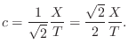
Discussion regarding solving the 2D wave equation subject to boundary conditions appears in §B.8.3. Interpreting this value for the wave propagation speed
The Lossy 2D Mesh
Because the finite-difference form of the digital waveguide mesh is the more efficient computationally than explicitly computing scattering wave variables (too see this, count the multiplies required per node), it is of interest to consider the finite-difference form also in the case of frequency-dependent losses. The method of §C.5.5 extends also to the waveguide mesh, which can be shown by generalizing the results of §C.14.4 above using the technique of §C.5.5.
The basic idea is once again that wave propagation during one sampling
interval (in time) is associated with linear filtering by ![]() .
That is,
.
That is, ![]() is regarded as the per-sample wave propagation filter.
is regarded as the per-sample wave propagation filter.
Diffuse Reflections in the Waveguide Mesh
In [416], Manfred Schroeder proposed the design of a
diffuse reflector based on a quadratic residue sequence. A
quadratic residue sequence ![]() corresponding to a prime number
corresponding to a prime number
![]() is the sequence
is the sequence ![]() mod
mod ![]() , for all integers
, for all integers ![]() . The sequence
is periodic with period
. The sequence
is periodic with period ![]() , so it is determined by
, so it is determined by ![]() for
for
![]() (i.e., one period of the infinite sequence).
(i.e., one period of the infinite sequence).
For example, when ![]() , the first period of the quadratic residue
sequence is given by
, the first period of the quadratic residue
sequence is given by
![\begin{eqnarray*}
a_7 &=& [0^2,1^2,2^2,3^2,4^2,5^2,6^2] \quad (\mbox{mod }7)\\
&=& [0, 1, 4, 2, 2, 4, 1]
\end{eqnarray*}](http://www.dsprelated.com/josimages_new/pasp/img4047.png)
An amazing property of these sequences is that their Fourier transforms have precisely constant magnitudes. That is, the sequence
![$\displaystyle \vert C_p(\omega_k)\vert \isdef \vert\dft _k(c_p)\vert
\isdef \l...
...^{p-1} c_p(n) e^{-j2\pi nk/p}\right\vert
= \sqrt{p}, \quad \forall k\in[0,p-1]
$](http://www.dsprelated.com/josimages_new/pasp/img4049.png)
Figure C.35 presents a simple matlab script which demonstrates the constant-magnitude Fourier property for all odd integers from 1 to 99.
function [c] = qrsfp(Ns)
%QRSFP Quadratic Residue Sequence Fourier Property demo
  if (nargin<1)
     Ns = 1:2:99; % Test all odd integers from 1 to 99
  end
  for N=Ns
    a = mod([0:N-1].^2,N);
    c = zeros(N-1,N);
    CM = zeros(N-1,N);
    c = exp(j*2*pi*a/N);
    CM = abs(fft(c))*sqrt(1/N);
    if (abs(max(CM)-1)>1E-10) || (abs(min(CM)-1)>1E-10)
       warn(sprintf("Failure for N=%d",N));
    end
  end
  r = exp(2i*pi*[0:100]/100); % a circle
  plot(real(r), imag(r),"k"); hold on;
  plot(c,"-*k"); % plot sequence in complex plane
end
|
Quadratic residue diffusers have been applied as boundaries of a 2D digital waveguide mesh in [279]. An article reviewing the history of room acoustic diffusers may be found in [94].
FDNs as Digital Waveguide Networks
This section supplements §2.7 on Feedback Delay Networks in the context of digital waveguide theory. Specifically, we review the interpretation of an FDN as a special case of a digital waveguide network, summarizing [463,464,385].
Figure C.36 illustrates an ![]() -branch DWN. It consists of a single
scattering junction, indicated by a white circle, to which
-branch DWN. It consists of a single
scattering junction, indicated by a white circle, to which ![]() branches are connected. The far end of each branch is terminated by an
ideal non-inverting reflection (black circle). The waves traveling
into the junction are associated with the FDN delay line outputs
branches are connected. The far end of each branch is terminated by an
ideal non-inverting reflection (black circle). The waves traveling
into the junction are associated with the FDN delay line outputs
![]() , and the length of each waveguide is
half the length of the corresponding FDN delay line
, and the length of each waveguide is
half the length of the corresponding FDN delay line ![]() (since a traveling wave must traverse the branch twice to complete a
round trip from the junction to the termination and back). When
(since a traveling wave must traverse the branch twice to complete a
round trip from the junction to the termination and back). When ![]() is odd, we may replace the reflecting termination by a unit-sample
delay.
is odd, we may replace the reflecting termination by a unit-sample
delay.
![\includegraphics[scale=0.5]{eps/DWN}](http://www.dsprelated.com/josimages_new/pasp/img4051.png) |
Lossless Scattering
The delay-line inputs (outgoing traveling waves) are computed by
multiplying the delay-line outputs (incoming traveling waves) by the
![]() feedback matrix (scattering matrix)
feedback matrix (scattering matrix)
![]() . By
defining
. By
defining
![]() ,
,
![]() , we obtain the more
usual DWN notation
, we obtain the more
usual DWN notation
where
The junction of ![]() physical waveguides determines the structure of the
matrix
physical waveguides determines the structure of the
matrix
![]() according to the basic principles of physics.
according to the basic principles of physics.
Considering the parallel junction of ![]() lossless acoustic tubes, each
having characteristic admittance
lossless acoustic tubes, each
having characteristic admittance
![]() , the continuity of pressure and
conservation of volume velocity at the junction give us the following
scattering matrix for the pressure waves [433]:
, the continuity of pressure and
conservation of volume velocity at the junction give us the following
scattering matrix for the pressure waves [433]:
![$\displaystyle {\bf A} = \left[ \begin{array}{rrrr} \frac{2 \Gamma_{1}}{\Gamma_J...
...{2}}{\Gamma_J} & \dots & \frac{2 \Gamma_{N}}{\Gamma_J} -1\\ \end{array} \right]$](http://www.dsprelated.com/josimages_new/pasp/img4059.png)
where
 |
(C.121) |
Equation (C.121) can be derived by first writing the volume velocity at the

Normalized Scattering
For ideal numerical scaling in the ![]() sense, we may choose to propagate
normalized waves which lead to normalized scattering junctions
analogous to those encountered in normalized ladder filters [297].
Normalized waves may be either normalized pressure
sense, we may choose to propagate
normalized waves which lead to normalized scattering junctions
analogous to those encountered in normalized ladder filters [297].
Normalized waves may be either normalized pressure
![]() or normalized velocity
or normalized velocity
![]() . Since the signal power associated with a traveling
wave is simply
. Since the signal power associated with a traveling
wave is simply
![]() ,
they may also be called root-power waves [432].
Appendix C develops this topic in more detail.
,
they may also be called root-power waves [432].
Appendix C develops this topic in more detail.
The scattering matrix for normalized pressure waves is given by
![$\displaystyle \tilde{\mathbf{A}}= \left[ \begin{array}{llll} \frac{2 \Gamma_{1}...
..._{2}}}{\Gamma_J} & \dots & \frac{2 \Gamma_{n}}{\Gamma_J} -1 \end{array} \right]$](http://www.dsprelated.com/josimages_new/pasp/img4066.png)
The normalized scattering matrix can be expressed as a negative Householder reflection
where
General Conditions for Losslessness
The scattering matrices for lossless physical waveguide junctions give an apparently unexplored class of lossless FDN prototypes. However, this is just a subset of all possible lossless feedback matrices. We are therefore interested in the most general conditions for losslessness of an FDN feedback matrix. The results below are adapted from [463,385].
Consider the general case in which
![]() is allowed to be any
scattering matrix, i.e., it is associated with a
not-necessarily-physical junction of
is allowed to be any
scattering matrix, i.e., it is associated with a
not-necessarily-physical junction of ![]() physical waveguides.
Following the definition of losslessness in classical network theory,
we may say that a waveguide scattering matrix
physical waveguides.
Following the definition of losslessness in classical network theory,
we may say that a waveguide scattering matrix
![]() is said to be
lossless if the total complex power
[35] at the junction is scattering invariant, i.e.,
is said to be
lossless if the total complex power
[35] at the junction is scattering invariant, i.e.,
where
The following theorem gives a general characterization of lossless scattering:
Theorem: A scattering matrix (FDN feedback matrix)
![]() is
lossless if and only if its eigenvalues lie on the unit circle and its
eigenvectors are linearly independent.
is
lossless if and only if its eigenvalues lie on the unit circle and its
eigenvectors are linearly independent.
Proof: Since
![]() is positive definite, it can be factored (by
the Cholesky factorization) into the form
is positive definite, it can be factored (by
the Cholesky factorization) into the form
![]() , where
, where
![]() is an upper triangular matrix, and
is an upper triangular matrix, and
![]() denotes the Hermitian
transpose of
denotes the Hermitian
transpose of
![]() , i.e.,
, i.e.,
![]() . Since
. Since
![]() is
positive definite,
is
positive definite,
![]() is nonsingular and can be used as a
similarity transformation matrix. Applying the Cholesky decomposition
is nonsingular and can be used as a
similarity transformation matrix. Applying the Cholesky decomposition
![]() in Eq.
in Eq.![]() (C.125) yields
(C.125) yields
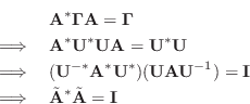
where
![]() , and
, and
Conversely, assume
![]() for each eigenvalue of
for each eigenvalue of
![]() , and
that there exists a matrix
, and
that there exists a matrix
![]() of linearly independent
eigenvectors of
of linearly independent
eigenvectors of
![]() . The matrix
. The matrix
![]() diagonalizes
diagonalizes
![]() to give
to give
![]() , where
, where
![]() diag
diag![]() . Taking the Hermitian transform of
this equation gives
. Taking the Hermitian transform of
this equation gives
![]() . Multiplying, we
obtain
. Multiplying, we
obtain
![]() . Thus, (C.125) is satisfied for
. Thus, (C.125) is satisfied for
![]() which is Hermitian and positive
definite.
which is Hermitian and positive
definite. ![]()
Thus, lossless scattering matrices may be fully parametrized as
![]() , where
, where
![]() is any unit-modulus diagonal
matrix, and
is any unit-modulus diagonal
matrix, and
![]() is any invertible matrix. In the real case, we
have
is any invertible matrix. In the real case, we
have
![]() diag
diag![]() and
and
![]() .
.
Note that not all lossless scattering matrices have a simple
physical interpretation as a scattering matrix for an
intersection of ![]() lossless reflectively terminated waveguides. In
addition to these cases (generated by all non-negative branch
impedances), there are additional cases corresponding to sign flips
and branch permutations at the junction. In terms of classical
network theory [35], such additional cases can be seen as
arising from the use of ``gyrators'' and/or ``circulators'' at the
scattering junction
[433]).
lossless reflectively terminated waveguides. In
addition to these cases (generated by all non-negative branch
impedances), there are additional cases corresponding to sign flips
and branch permutations at the junction. In terms of classical
network theory [35], such additional cases can be seen as
arising from the use of ``gyrators'' and/or ``circulators'' at the
scattering junction
[433]).
Waveguide Transformers and Gyrators
The ideal transformer, depicted in Fig. C.37 a, is a
lossless two-port electric circuit element which scales up voltage by
a constant ![]() [110,35]. In other words, the voltage at
port 2 is always
[110,35]. In other words, the voltage at
port 2 is always ![]() times the voltage at port 1. Since power is
voltage times current, the current at port 2 must be
times the voltage at port 1. Since power is
voltage times current, the current at port 2 must be ![]() times the
current at port 1 in order for the transformer to be lossless. The
scaling constant
times the
current at port 1 in order for the transformer to be lossless. The
scaling constant ![]() is called the turns ratio because
transformers are built by coiling wire around two sides of a
magnetically permeable torus, and the number of winds around the port
2 side divided by the winding count on the port 1 side gives the
voltage stepping constant
is called the turns ratio because
transformers are built by coiling wire around two sides of a
magnetically permeable torus, and the number of winds around the port
2 side divided by the winding count on the port 1 side gives the
voltage stepping constant ![]() .
.
![\includegraphics[width=\twidth]{eps/lTransformer}](http://www.dsprelated.com/josimages_new/pasp/img4102.png) |
In the case of mechanical circuits, the two-port transformer relations appear as
![\begin{eqnarray*}
F_2(s) &=& g F_1(s) \\ [5pt]
V_2(s) &=& \frac{1}{g} V_1(s)
\end{eqnarray*}](http://www.dsprelated.com/josimages_new/pasp/img4103.png)
where ![]() and
and ![]() denote force and velocity, respectively.
We now convert these transformer describing
equations to the wave variable formulation. Let
denote force and velocity, respectively.
We now convert these transformer describing
equations to the wave variable formulation. Let ![]() and
and ![]() denote
the wave impedances on the port 1 and port 2 sides,
respectively, and define velocity as positive into the transformer. Then
denote
the wave impedances on the port 1 and port 2 sides,
respectively, and define velocity as positive into the transformer. Then
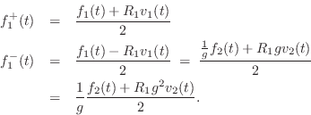
Similarly,
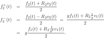
We see that choosing

![\begin{eqnarray*}
f^{{-}}_2(t) &=& g f^{{+}}_1(t)\\ [5pt]
f^{{-}}_1(t) &=& \frac{1}{g}f^{{+}}_2(t).
\end{eqnarray*}](http://www.dsprelated.com/josimages_new/pasp/img4107.png)
The corresponding wave flow diagram is shown in Fig. C.37 b.
Thus, a transformer with a voltage gain ![]() corresponds to simply
changing the wave impedance from
corresponds to simply
changing the wave impedance from ![]() to
to ![]() , where
, where
![]() . Note that the transformer implements a change
in wave impedance without scattering as occurs in physical
impedance steps (§C.8).
. Note that the transformer implements a change
in wave impedance without scattering as occurs in physical
impedance steps (§C.8).
Gyrators
Another way to define the ideal waveguide transformer is to ask for a
two-port element that joins two waveguide sections of differing wave
impedance in such a way that signal power is preserved and no
scattering occurs. From Ohm's Law for traveling waves
(Eq.![]() (6.6)), and from the definition of power waves
(§C.7.5), we see that to bridge an impedance
discontinuity between
(6.6)), and from the definition of power waves
(§C.7.5), we see that to bridge an impedance
discontinuity between ![]() and
and ![]() with no power change and no scattering requires the
relations
with no power change and no scattering requires the
relations
![$\displaystyle \frac{[f^{{+}}_i]^2}{R_i} = \frac{[f^{{+}}_{i-1}]^2}{R_{i-1}}, \qquad\qquad
\frac{[f^{{-}}_i]^2}{R_i} = \frac{[f^{{-}}_{i-1}]^2}{R_{i-1}}.
$](http://www.dsprelated.com/josimages_new/pasp/img4109.png)
where
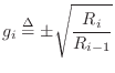
Choosing the negative square root for
The dualizer is readily derived from Ohm's Law for traveling waves:
![\begin{eqnarray*}
f^{{+}}\eqsp Rv^{+}, \qquad
f^{{-}}\eqsp -Rv^{-}\\ [5pt]
\Lon...
...i\eqsp Rv^{+}_{i-1}, \qquad
v^{-}_{i-1} \eqsp -R^{-1} f^{{-}}_i
\end{eqnarray*}](http://www.dsprelated.com/josimages_new/pasp/img4112.png)
In this case, velocity waves in section ![]() are converted to force
waves in section
are converted to force
waves in section ![]() , and vice versa (all at wave impedance
, and vice versa (all at wave impedance ![]() ). The
wave impedance can be changed as well by cascading a transformer with
the dualizer, which changes
). The
wave impedance can be changed as well by cascading a transformer with
the dualizer, which changes ![]() to
to
![]() (where we assume
(where we assume ![]() ). Finally, the velocity waves in section
). Finally, the velocity waves in section
![]() can be scaled to equal their corresponding force waves by
introducing a transformer
can be scaled to equal their corresponding force waves by
introducing a transformer
![]() on the left, which then
coincides Eq.
on the left, which then
coincides Eq.![]() (C.126) (but with a minus sign in the second equation).
(C.126) (but with a minus sign in the second equation).
The Digital Waveguide Oscillator
In this section, adapted from [460], a digital sinusoidal oscillator derived from digital waveguide theory is described which has good properties for VLSI implementation. Its main features are no wavetable and a computational complexity of only one multiply per sample when amplitude and frequency are constant. Three additions are required per sample. A piecewise exponential amplitude envelope is available for the cost of a second multiplication per sample, which need not be as expensive as the tuning multiply. In the presence of frequency modulation (FM), the amplitude coefficient can be varied to exactly cancel amplitude modulation (AM) caused by changing the frequency of oscillation.
Additive Synthesis
One of the very first computer music techniques introduced was additive synthesis [379]. It is based on Fourier's theorem which states that any sound can be constructed from elementary sinusoids, such as are approximately produced by carefully struck tuning forks. Additive synthesis attempts to apply this theorem to the synthesis of sound by employing large banks of sinusoidal oscillators, each having independent amplitude and frequency controls. Many analysis methods, e.g., the phase vocoder, have been developed to support additive synthesis. A summary is given in [424].
While additive synthesis is very powerful and general, it has been held
back from widespread usage due to its computational expense. For example,
on a single DSP56001 digital signal-processing chip, clocked at 33 MHz,
only about ![]() sinusoidal partials can be synthesized in real time using
non-interpolated, table-lookup oscillators. Interpolated table-lookup
oscillators are much more expensive, and when all the bells and whistles
are added, and system overhead is accounted for, only around
sinusoidal partials can be synthesized in real time using
non-interpolated, table-lookup oscillators. Interpolated table-lookup
oscillators are much more expensive, and when all the bells and whistles
are added, and system overhead is accounted for, only around ![]() fully
general, high-quality partials are sustainable at
fully
general, high-quality partials are sustainable at ![]() KHz on a
KHz on a ![]() DSP56001 (based on analysis of implementations provided by the NeXT Music
Kit).
DSP56001 (based on analysis of implementations provided by the NeXT Music
Kit).
At CD-quality sampling rates, the note A1 on the piano requires
![]() sinusoidal partials, and at least the low-frequency
partials should use interpolated lookups. Assuming a worst-case average of
sinusoidal partials, and at least the low-frequency
partials should use interpolated lookups. Assuming a worst-case average of
![]() partials per voice, providing 32-voice polyphony requires
partials per voice, providing 32-voice polyphony requires ![]() partials, or around
partials, or around ![]() DSP chips, assuming we can pack an average of
DSP chips, assuming we can pack an average of ![]() partials into each DSP. A more reasonable complement of
partials into each DSP. A more reasonable complement of ![]() DSP chips
would provide only
DSP chips
would provide only ![]() -voice polyphony which is simply not enough for a
piano synthesis. However, since DSP chips are getting faster and cheaper,
DSP-based additive synthesis looks viable in the future.
-voice polyphony which is simply not enough for a
piano synthesis. However, since DSP chips are getting faster and cheaper,
DSP-based additive synthesis looks viable in the future.
The cost of additive synthesis can be greatly reduced by making special purpose VLSI optimized for sinusoidal synthesis. In a VLSI environment, major bottlenecks are wavetables and multiplications. Even if a single sinusoidal wavetable is shared, it must be accessed sequentially, inhibiting parallelism. The wavetable can be eliminated entirely if recursive algorithms are used to synthesize sinusoids directly.
Digital Sinusoid Generators
In [168], three techniques were examined for generating sinusoids digitally by means of recursive algorithms.C.12 The recursions can be interpreted as implementations of second-order digital resonators in which the damping is set to zero. The three methods considered were (1) the 2D rotation (2DR), or complex multiply (also called the ``coupled form''), (2) the modified coupled form (MCF), or ``magic circle'' algorithm,C.13which is similar to (1) but with better numerical behavior, and (3) the direct-form, second-order, digital resonator (DFR) with its poles set to the unit circle.
These three recursions may be defined as follows:
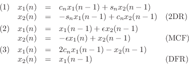
The digital waveguide oscillator appears to have the best overall properties yet seen for VLSI implementation. This structure, introduced in [460], may be derived from the theory of digital waveguides (see Appendix C, particularly §C.9, and [433,464]). Any second-order digital filter structure can be used as a starting point for developing a corresponding sinusoidal signal generator, so in this case we begin with the second-order waveguide filter.
The Second-Order Waveguide Filter
The first step is to make a second-order digital filter with zero
damping by abutting two unit-sample sections of waveguide medium, and
terminating on the left and right with perfect reflections, as shown
in Fig.C.38. The wave impedance in section ![]() is given by
is given by
![]() , where
, where ![]() is air density,
is air density, ![]() is the
cross-sectional area of tube section
is the
cross-sectional area of tube section ![]() , and
, and ![]() is sound speed. The
reflection coefficient is determined by the impedance discontinuity
via
is sound speed. The
reflection coefficient is determined by the impedance discontinuity
via
![]() . It turns out that to obtain sinusoidal
oscillation, one of the terminations must provide an inverting
reflection while the other is non-inverting.
. It turns out that to obtain sinusoidal
oscillation, one of the terminations must provide an inverting
reflection while the other is non-inverting.
![\includegraphics[width=\twidth]{eps/wgf}](http://www.dsprelated.com/josimages_new/pasp/img4129.png) |
At the junction between sections ![]() and
and ![]() , the signal is partially
transmitted and partially reflected such that energy is conserved, i.e., we
have lossless scattering. The formula for the reflection
coefficient
, the signal is partially
transmitted and partially reflected such that energy is conserved, i.e., we
have lossless scattering. The formula for the reflection
coefficient ![]() can be derived from the physical constraints that (1)
pressure is continuous across the junction, and (2) there is no net flow
into or out of the junction. For traveling pressure waves
can be derived from the physical constraints that (1)
pressure is continuous across the junction, and (2) there is no net flow
into or out of the junction. For traveling pressure waves ![]() and
volume-velocity waves
and
volume-velocity waves ![]() , we have
, we have
![]() and
and
![]() . The physical pressure and volume velocity are obtained by
summing the traveling-wave components.
. The physical pressure and volume velocity are obtained by
summing the traveling-wave components.
The discrete-time simulation for the physical system of Fig.C.38 is shown in Fig.C.39. The propagation time from the junction to a reflecting termination and back is one sample period. The half sample delay from the junction to the reflecting termination has been commuted with the termination and combined with the half sample delay to the termination. This is a special case of a ``half-rate'' waveguide filter [433].
![\includegraphics[width=\twidth]{eps/dwgf}](http://www.dsprelated.com/josimages_new/pasp/img4134.png)
Since only two samples of delay are present, the digital system is at most
second order, and since the coefficients are real, at most one frequency of
oscillation is possible in ![]() .
.
The scattering junction shown in the figure is called the Kelly-Lochbaum junction in the literature on lattice and ladder digital filters [173]. While it is the most natural from a physical point of view, it requires four multiplies and two additions for its implementation.
It is well known that lossless scattering junctions can be implemented in a
variety of equivalent forms, such as the two-multiply and even one-multiply
junctions. However, most have the disadvantage of not being normalized in the sense that changing the reflection coefficient ![]() changes the amplitude of oscillation. This can be understood physically by
noting that a change in
changes the amplitude of oscillation. This can be understood physically by
noting that a change in ![]() implies a change in
implies a change in ![]() . Since the
signal power contained in a waveguide variable, say
. Since the
signal power contained in a waveguide variable, say ![]() , is
, is
![]() , we find that modulating the reflection coefficient
corresponds to modulating the signal energy represented by the signal
sample in at least one of the two delay elements. Since energy is
proportional to amplitude squared, energy modulation implies amplitude
modulation.
, we find that modulating the reflection coefficient
corresponds to modulating the signal energy represented by the signal
sample in at least one of the two delay elements. Since energy is
proportional to amplitude squared, energy modulation implies amplitude
modulation.
The well-known normalization procedure is to replace the traveling
pressure waves ![]() by ``root-power'' pressure waves
by ``root-power'' pressure waves
![]() so that signal power is just the square of a signal
sample
so that signal power is just the square of a signal
sample
![]() . When this is done, the scattering junction
transforms from the Kelly-Lochbaum or one-multiply form into the
normalized ladder junction in which the reflection coefficients
are again
. When this is done, the scattering junction
transforms from the Kelly-Lochbaum or one-multiply form into the
normalized ladder junction in which the reflection coefficients
are again ![]() , but the forward and reverse transmission
coefficients become
, but the forward and reverse transmission
coefficients become
![]() . Defining
. Defining
![]() , the
transmission coefficients can be seen as
, the
transmission coefficients can be seen as
![]() , and we arrive
essentially at the coupled form, or two-dimensional vector
rotation considered in [168].
, and we arrive
essentially at the coupled form, or two-dimensional vector
rotation considered in [168].
An alternative normalization technique is based on the digital waveguide
transformer (§C.16). The purpose of a ``transformer'' is to
``step'' the force variable (pressure in our example) by some factor ![]() without scattering and without affecting signal energy. Since traveling
signal power is proportional to pressure times velocity
without scattering and without affecting signal energy. Since traveling
signal power is proportional to pressure times velocity ![]() , it
follows that velocity must be stepped by the inverse factor
, it
follows that velocity must be stepped by the inverse factor ![]() to keep
power constant. This is the familiar behavior of transformers for analog
electrical circuits: voltage is stepped up by the ``turns ratio'' and
current is stepped down by the reciprocal factor. Now, since
to keep
power constant. This is the familiar behavior of transformers for analog
electrical circuits: voltage is stepped up by the ``turns ratio'' and
current is stepped down by the reciprocal factor. Now, since
![]() , traveling signal power is equal to
, traveling signal power is equal to
![]() . Therefore,
stepping up pressure through a transformer by the factor
. Therefore,
stepping up pressure through a transformer by the factor ![]() corresponds to
stepping up the wave impedance
corresponds to
stepping up the wave impedance ![]() by the factor
by the factor ![]() . In other words,
the transformer raises pressure and decreases volume velocity by raising
the wave impedance (narrowing the acoustic tube) like a converging cone.
. In other words,
the transformer raises pressure and decreases volume velocity by raising
the wave impedance (narrowing the acoustic tube) like a converging cone.
If a transformer is inserted in a waveguide immediately to the left, say,
of a scattering junction, it can be used to modulate the wave impedance
``seen'' to the left by the junction without having to use root-power waves
in the simulation. As a result, the one-multiply junction can be used for
the scattering junction, since the junction itself is not normalized.
Since the transformer requires two multiplies, a total of three multiplies
can effectively implement a normalized junction, where four were needed
before. Finally, in just this special case, one of the transformer
coefficients can be commuted with the delay element on the left and
combined with the other transformer coefficient. For convenience, the ![]() coefficient on the left is commuted into the junction so it merely toggles
the signs of inputs to existing summers. These transformations lead to the
final form shown in Fig.C.40.
coefficient on the left is commuted into the junction so it merely toggles
the signs of inputs to existing summers. These transformations lead to the
final form shown in Fig.C.40.
![\includegraphics[scale=0.9]{eps/tnwgoAI}](http://www.dsprelated.com/josimages_new/pasp/img4149.png)
The ``tuning coefficient'' is given by
![]() , where
, where
![]() is the desired oscillation frequency in Hz at sample
is the desired oscillation frequency in Hz at sample ![]() (in the
undamped case), and
(in the
undamped case), and ![]() is the sampling period in seconds. The
``amplitude coefficient'' is
is the sampling period in seconds. The
``amplitude coefficient'' is
![]() , where growth or
decay factor per sample (
, where growth or
decay factor per sample (
![]() for constant
amplitude),C.14 and
for constant
amplitude),C.14 and ![]() is the normalizing transformer ``turns
ratio'' given by
is the normalizing transformer ``turns
ratio'' given by
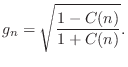
When amplitude and frequency are constant, there is no gradual exponential
growth or decay due to round-off error. This happens because the only
rounding is at the output of the tuning multiply, and all other
computations are exact. Therefore, quantization in the tuning coefficient
can only cause quantization in the frequency of oscillation. Note that any
one-multiply digital oscillator should have this property. In contrast,
the only other known normalized oscillator, the coupled form, does
exhibit exponential amplitude drift because it has two coefficients
![]() and
and
![]() which, after quantization, no longer
obey
which, after quantization, no longer
obey ![]() for most tunings.
for most tunings.
Application to FM Synthesis
The properties of the new oscillator appear well suited for FM
applications in VLSI because of the minimized computational expense.
However, in this application there are issues to be resolved regarding
conversion from modulator output to carrier coefficients. Preliminary
experiments indicate that FM indices less than ![]() are well behaved
when the output of a modulating oscillator simply adds to the
coefficient of the carrier oscillator (bypassing the exact FM
formulas). Approximate amplitude normalizing coefficients have also
been derived which provide a first-order approximation to the exact AM
compensation at low cost. For music synthesis applications, we
believe a distortion in the details of the FM instantaneous frequency
trajectory and a moderate amount of incidental AM can be tolerated
since they produce only second-order timbral effects in many
situations.
are well behaved
when the output of a modulating oscillator simply adds to the
coefficient of the carrier oscillator (bypassing the exact FM
formulas). Approximate amplitude normalizing coefficients have also
been derived which provide a first-order approximation to the exact AM
compensation at low cost. For music synthesis applications, we
believe a distortion in the details of the FM instantaneous frequency
trajectory and a moderate amount of incidental AM can be tolerated
since they produce only second-order timbral effects in many
situations.
Digital Waveguide Resonator
Converting a second-order oscillator into a second-order filter
requires merely introducing damping and defining the input and output
signals. In Fig.C.40, damping is provided by the coefficient
![]() , which we will take to be a constant
, which we will take to be a constant
The foregoing modifications to the digital waveguide oscillator result
in the so-called digital waveguide resonator (DWR)
[304]:
where, as derived in the next section, the coefficients are given by

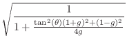
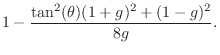
where
Figure C.41 shows an overlay of initial impulse responses for
the three resonators discussed above. The decay factor was set to
![]() , and the output of each multiplication was quantized to 16
bits, as were all coefficients. The three waveforms sound and look
identical. (There are small differences, however, which can be
seen by plotting the differences of pairs of waveforms.)
, and the output of each multiplication was quantized to 16
bits, as were all coefficients. The three waveforms sound and look
identical. (There are small differences, however, which can be
seen by plotting the differences of pairs of waveforms.)
![\includegraphics[width=\twidth]{eps/tosc16}](http://www.dsprelated.com/josimages_new/pasp/img4188.png) |
Figure C.42 shows the same impulse-response overlay but with
![]() and only 4 significant bits in the coefficients and signals.
The complex multiply oscillator can be seen to decay toward zero due
to coefficient quantization (
and only 4 significant bits in the coefficients and signals.
The complex multiply oscillator can be seen to decay toward zero due
to coefficient quantization (
![]() ). The MCF and DWR remain
steady at their initial amplitude. All three suffer some amount of
tuning perturbation.
). The MCF and DWR remain
steady at their initial amplitude. All three suffer some amount of
tuning perturbation.
![\includegraphics[width=\twidth]{eps/tosc4}](http://www.dsprelated.com/josimages_new/pasp/img4190.png) |
State-Space Analysis
We will now use state-space analysisC.15[449] to determine Equations (C.133-C.136).
![$\displaystyle \left[\begin{array}{c} x_1(n+1) \\ [2pt] x_2(n+1) \end{array}\rig...
...bf{A} \left[\begin{array}{c} x_1(n) \\ [2pt] x_2(n) \end{array}\right] \protect$](http://www.dsprelated.com/josimages_new/pasp/img4193.png)
or, in vector notation,
| (C.137) | |||
| (C.138) |
where we have introduced an input signal
A basic fact from linear algebra is that the determinant of a
matrix is equal to the product of its eigenvalues. As a quick
check, we find that the determinant of ![]() is
is
When the eigenvalues
Note that
![]() . If we diagonalize this system to
obtain
. If we diagonalize this system to
obtain
![]() , where
, where
![]() diag
diag![]() , and
, and
![]() is the matrix of eigenvectors
of
is the matrix of eigenvectors
of
![]() , then we have
, then we have
![$\displaystyle \tilde{\underline{x}}(n) = \tilde{A}^n\,\tilde{\underline{x}}(0) ...
...eft[\begin{array}{c} \tilde{x}_1(0) \\ [2pt] \tilde{x}_2(0) \end{array}\right]
$](http://www.dsprelated.com/josimages_new/pasp/img4209.png)
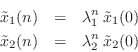
If this system is to generate a real sampled sinusoid at radian frequency
![]() , the eigenvalues
, the eigenvalues ![]() and
and ![]() must be of the form
must be of the form
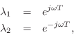
(in either order) where ![]() is real, and
is real, and ![]() denotes the sampling
interval in seconds.
denotes the sampling
interval in seconds.
Thus, we can determine the frequency of oscillation ![]() (and
verify that the system actually oscillates) by determining the
eigenvalues
(and
verify that the system actually oscillates) by determining the
eigenvalues ![]() of
of ![]() . Note that, as a prerequisite, it will
also be necessary to find two linearly independent eigenvectors of
. Note that, as a prerequisite, it will
also be necessary to find two linearly independent eigenvectors of ![]() (columns of
(columns of
![]() ).
).
Eigenstructure
Starting with the defining equation for an eigenvector
![]() and its
corresponding eigenvalue
and its
corresponding eigenvalue ![]() ,
,
![$\displaystyle \left[\begin{array}{cc} gc & c-1 \\ [2pt] gc+g & c \end{array}\ri...
...n{array}{c} {\lambda_i} \\ [2pt] {\lambda_i}\eta_i \end{array}\right]. \protect$](http://www.dsprelated.com/josimages_new/pasp/img4218.png)
We normalized the first element of
Equation (C.141) gives us two equations in two unknowns:
Substituting the first into the second to eliminate
![\begin{eqnarray*}
g+gc+c\eta_i &=& [gc+\eta_i(c-1)]\eta_i = gc\eta_i + \eta_i^2 ...
...{g\left(\frac{1+c}{1-c}\right)
- \frac{c^2(1-g)^2}{4(1-c)^2}}.
\end{eqnarray*}](http://www.dsprelated.com/josimages_new/pasp/img4224.png)
As ![]() approaches
approaches ![]() (no damping), we obtain
(no damping), we obtain
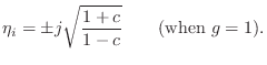
![\begin{eqnarray*}
\underline{e}_1&=&\left[\begin{array}{c} 1 \\ [2pt] \eta \end{...
...t{g\left(\frac{1+c}{1-c}\right)
- \frac{c^2(1-g)^2}{4(1-c)^2}}
\end{eqnarray*}](http://www.dsprelated.com/josimages_new/pasp/img4226.png)
They are linearly independent provided ![]() . In the undamped
case (
. In the undamped
case (![]() ), this holds whenever
), this holds whenever ![]() . The eigenvectors are
finite when
. The eigenvectors are
finite when ![]() . Thus, the nominal range for
. Thus, the nominal range for ![]() is the
interval
is the
interval
![]() .
.
We can now use Eq.![]() (C.142) to find the eigenvalues:
(C.142) to find the eigenvalues:
![\begin{eqnarray*}
{\lambda_i}&=& gc+ \eta_i(c-1)\\
&=& gc+ \frac{(1-g)c}{2}\pm ...
...
\pm j\sqrt{g(1-c^2) - \left[\frac{c(1-g)}{2}\right]^2}
\protect
\end{eqnarray*}](http://www.dsprelated.com/josimages_new/pasp/img4231.png)
Damping and Tuning Parameters
The tuning and damping of the resonator impulse response are governed by the relation
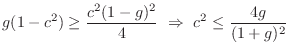
To obtain a specific decay time-constant ![]() , we must have
, we must have
![\begin{eqnarray*}
e^{-2T/\tau} &=& \left\vert{\lambda_i}\right\vert^2 = c^2\left...
...left[g(1-c^2) - c^2\left(\frac{1-g}{2}\right)^2\right]\\
&=& g
\end{eqnarray*}](http://www.dsprelated.com/josimages_new/pasp/img4234.png)
Therefore, given a desired decay time-constant ![]() (and the
sampling interval
(and the
sampling interval ![]() ), we may compute the damping parameter
), we may compute the damping parameter ![]() for
the digital waveguide resonator as
for
the digital waveguide resonator as
To obtain a desired frequency of oscillation, we must solve
![\begin{eqnarray*}
\theta = \omega T
&=& \tan^{-1}\left[\frac{\sqrt{g(1-c^2) - [...
...,\tan^2{\theta} &=& \frac{g(1-c^2) - [c(1-g)/2]^2}{[c(1+g)/2]^2}
\end{eqnarray*}](http://www.dsprelated.com/josimages_new/pasp/img4236.png)
for ![]() , which yields
, which yields
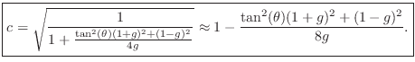
Eigenvalues in the Undamped Case
When ![]() , the eigenvalues reduce to
, the eigenvalues reduce to
where
For
![]() , the eigenvalues are real, corresponding to
exponential growth and/or decay. (The values
, the eigenvalues are real, corresponding to
exponential growth and/or decay. (The values ![]() were
excluded above in deriving Eq.
were
excluded above in deriving Eq.![]() (C.144).)
(C.144).)
In summary, the coefficient ![]() in the digital waveguide oscillator
(
in the digital waveguide oscillator
(![]() ) and the frequency of sinusoidal oscillation
) and the frequency of sinusoidal oscillation ![]() is simply
is simply
Summary
This section introduced and analyzed the digital waveguide oscillator and resonator, as well as some related algorithms. As a recursive algorithm for digital sinusoid generation, it has excellent properties for VLSI implementation. It is like the 2D rotation (complex multiply) in that it offers instantaneous amplitude from its state and constant amplitude in the presence of frequency modulation. However, its implementation requires only two multiplies per sample instead of four. When used as a constant-frequency oscillator, it requires only one multiply per sample.
Matlab Sinusoidal Oscillator Implementations
This section provides Matlab/Octave program listings for the sinusoidal resonator/oscillator algorithms discussed above:
- Planar 2D Rotation (2DR) (``complex multiply'')
- Modified Coupled Form (MCF) (``Magic Circle'')
- Digital Waveguide Resonator (DWR)
% Filter test program in matlab

%N = 300;   % Number of samples to generate
N = 3000;   % Number of samples to generate
f = 100;   % Desired oscillation frequency (Hz)
fs = 8192; % Audio sampling rate (Hz)
%R = .99;   % Decay factor (1=never, 0=instant)
R = 1;   % Decay factor (1=never, 0=instant)
b1 = 1;    % Input gain to state variable x(n)
b2 = 0;    % Input gain to state variable y(n)

%nd = 16;   % Number of significant digits to use
nd = 4;   % Number of significant digits to use
base = 2;  % Mantissa base (two significant figures)
           % (see 'help chop' in Matlab)

u = [1,zeros(1,N-1)]; % driving input test signal
theta = 2*pi*f/fs; % resonance frequency, rad/sample

% ================================================
% 2D PLANAR ROTATION (COMPLEX MULTIPLY)

x1 = zeros(1,N); % Predeclare saved-state arrays
y1 = zeros(1,N);

x1(1) = 0;      % Initial condition
y1(1) = 0;      % Initial condition

c = chop(R*cos(theta),nd,base); % coefficient 1
s = chop(R*sin(theta),nd,base); % coefficient 2

for n=1:N-1,
  x1(n+1) = chop(   c*x1(n) - s*y1(n) + b1*u(n), nd,base);
  y1(n+1) = chop(   s*x1(n) + c*y1(n) + b2*u(n), nd,base);
end

% ================================================
% MODIFIED COUPLED FORM ("MAGIC CIRCLE")
% (ref: http://ccrma.stanford.edu/~jos/wgo/ )

x2 = zeros(1,N); % Predeclare saved-state arrays
y2 = zeros(1,N);

x2(1) = 0.0;     % Initial condition
y2(1) = 0.0;     % Initial condition

e = chop(2*sin(theta/2),nd,base); % tuning coefficient

for n=1:N-1,
  x2(n+1) = chop(R*(x2(n)-e*y2(n))+b1*u(n),nd,base);
  y2(n+1) = chop(R*(e*x2(n+1)+y2(n))+b2*u(n),nd,base);
end

% ================================================
% DIGITAL WAVEGUIDE RESONATOR (DWR)

x3 = zeros(1,N); % Predeclare saved-state arrays
y3 = zeros(1,N);

x3(1) = 0;      % Initial condition
y3(1) = 0;      % Initial condition

g = R*R;        % decay coefficient
t = tan(theta); % toward tuning coefficient
cp = sqrt(g/(g + t^2*(1+g)^2/4 + (1-g)^2/4)); % exact
%cp = 1 - (t^2*(1+g)^2 + (1-g)^2)/(8*g); % good approx
b1n = b1*sqrt((1-cp)/(1+cp)); % input scaling

% Quantize coefficients:
cp = chop(cp,nd,base);
g = chop(g,nd,base);
b1n = chop(b1n,nd,base);

for n=1:N-1,
  gx3 = chop(g*x3(n), nd,base); % mpy 1
  y3n = y3(n);
  temp = chop(cp*(gx3 + y3n), nd,base); % mpy 2
  x3(n+1) = temp - y3n + b1n*u(n);
  y3(n+1) = gx3 + temp + b2*u(n);
end

% ================================================
% playandplot.m

figure(4);
title('Impulse Response Overlay');
ylabel('Amplitude');
xlabel('Time (samples)');
alt=1;%alt = (-1).^(0:N-1); % for visibility
plot([y1',y2',(alt.*y3)']); grid('on');
legend('2DR','MCF','WGR');
title('Impulse Response Overlay');
ylabel('Amplitude');
xlabel('Time (samples)');

saveplot(sprintf('eps/tosc%d.ps',nd));

if 1
  playandplot(y1,u,fs,'2D rotation',1);
  playandplot(y2,u,fs,'Magic circle',2);
  playandplot(y3,u,fs,'WGR',3);
end

function playandplot(y,u,fs,ttl,fnum);
% sound(y,fs,16);
  figure(fnum);

  unwind_protect # protect graph state
  subplot(211);
  axis("labely");
  axis("autoy");
  xlabel("");
  title(ttl);
  ylabel('Amplitude');
  xlabel('Time (ms)');
  t = 1000*(0:length(u)-1)/fs;
  timeplot(t,u,'-');
  legend('input');
  subplot(212);
  ylabel('Amplitude');
  xlabel('Time (ms)');
  timeplot(t,y,'-');
  legend('output');
  unwind_protect_cleanup # restore graph state
    grid("off");
    axis("auto","label");
    oneplot();
  end_unwind_protect
endfunction
Note that the chop utility only exists in Matlab. In Octave, the following ``compatibility stub'' can be used:
function [y] = chop(x,nd,base)
y = x;
Faust Implementation
The function oscw (file osc.lib) implements a digital waveguide sinusoidal oscillator in the Faust language [453,154,170]. There is also oscr implementing the 2D rotation case, and oscs implementing the modified coupled form (magic circle).
Non-Cylindrical Acoustic Tubes
In many situations, the wave impedance of the medium varies in a continuous manner rather than in discrete steps. This occurs, for example, in conical bores and flaring horns. In this section, based on [436], we will consider non-cylindrical acoustic tubes.
Horns as Waveguides
Waves in a horn can be analyzed as one-parameter waves, meaning that it is assumed that a constant-phase wavefront progresses uniformly along the horn. Each ``surface of constant phase'' composing the traveling wave has tangent planes normal to the horn axis and to the horn boundary. For cylindrical tubes, the surfaces of constant phase are planar, while for conical tubes, they are spherical [357,317,144]. The key property of a ``horn'' is that a traveling wave can propagate from one end to the other with negligible ``backscattering'' of the wave. Rather, it is smoothly ``guided'' from one end to the other. This is the meaning of saying that a horn is a ``waveguide''. The absence of backscattering means that the entire propagation path may be simulated using a pure delay line, which is very efficient computationally. Any losses, dispersion, or amplitude change due to horn radius variation (``spreading loss'') can be implemented where the wave exits the delay line to interact with other components.
Overview of Methods
We will first consider the elementary case of a conical acoustic tube. All smooth horns reduce to the conical case over sufficiently short distances, and the use of many conical sections, connected via scattering junctions, is often used to model an arbitrary bore shape [71]. The conical case is also important because it is essentially the most general shape in which there are exact traveling-wave solutions (spherical waves) [357].
Beyond conical bore shapes, however, one can use a Sturm-Liouville formulation to solve for one-parameter-wave scattering parameters [50]. In this formulation, the curvature of the bore's cross-section (more precisely, the curvature of the one-parameter wave's constant-phase surface area) is treated as a potential function that varies along the horn axis, and the solution is an eigenfunction of this potential. Sturm-Liouville analysis is well known in quantum mechanics for solving elastic scattering problems and for finding the wave functions (at various energy levels) for an electron in a nonuniform potential well.
When the one-parameter-wave assumption breaks down, and multiple acoustic modes are excited, the boundary element method (BEM) is an effective tool [190]. The BEM computes the acoustic field from velocity data along any enclosing surface. There also exist numerical methods for simulating wave propagation in varying cross-sections that include ``mode conversion'' [336,13,117].
This section will be henceforth concerned with non-cylindrical tubes in which backscatter and mode-conversion can be neglected, as treated in [317]. The only exact case is the cone, but smoothly varying horn shapes can be modeled approximately in this way.
Back to the Cone
Note that the cylindrical tube is a limiting case of a cone with its apex at infinity. Correspondingly, a plane wave is a limiting case of a spherical wave having infinite radius.
On a fundamental level, all pressure waves in 3D space are composed of spherical waves [357]. You may have learned about the Huygens-Fresnel principle in a physics class when it covered waves [295]. The Huygens-Fresnel principle states that the propagation of any wavefront can be modeled as the superposition of spherical waves emanating from all points along the wavefront [122, page 344]. This principle is especially valuable for intuitively understanding diffraction and related phenomena such as mode conversion (which happens, for example, when a plane wave in a horn hits a sharp bend or obstruction and breaks up into other kinds of waves in the horn).
Conical Acoustic Tubes
The conical acoustic tube is a one-dimensional waveguide which propagates circular sections of spherical pressure waves in place of the plane wave which traverses a cylindrical acoustic tube [22,349]. The wave equation in the spherically symmetric case is given by
where
Spherical coordinates are appropriate because simple closed-form
solutions to the wave equation are only possible when the forced boundary
conditions lie along coordinate planes. In the case of a cone, the
boundary conditions lie along a conical section of a sphere. It can be
seen that the wave equation in a cone is identical to the wave equation in
a cylinder, except that ![]() is replaced by
is replaced by ![]() . Thus, the solution is a
superposition of left- and right-going traveling wave components, scaled by
. Thus, the solution is a
superposition of left- and right-going traveling wave components, scaled by
![]() :
:
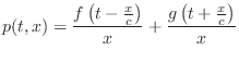
where
In cylindrical tubes, the velocity wave is in phase with the pressure wave. This is not the case with conical or more general tubes. The velocity of a traveling may be computed from the corresponding traveling pressure wave by dividing by the wave impedance.
Digital Simulation
A discrete-time simulation of the above solution may be obtained by simply
sampling the traveling-wave amplitude at intervals of ![]() seconds, which implies a spatial sampling interval of
seconds, which implies a spatial sampling interval of
![]() meters. Sampling is carried out mathematically by the
change of variables
meters. Sampling is carried out mathematically by the
change of variables
![\begin{eqnarray*}
x_mp(t_n,x_m) &\,\mathrel{\mathop=}\,& f(t_n- x_m/c)+g(t_n+ x...
...hop=}\,& f\left[(n-m)T-x_0/c\right]+ g\left[(n+m)T+x_0/c\right].
\end{eqnarray*}](http://www.dsprelated.com/josimages_new/pasp/img4258.png)
Define
![\includegraphics[width=\twidth]{eps/fcideal}](http://www.dsprelated.com/josimages_new/pasp/img4261.png) |
A more compact simulation diagram which stands for either sampled or continuous simulation is shown in Figure C.44. The figure emphasizes that the ideal, lossless waveguide is simulated by a bidirectional delay line.
![\includegraphics[width=\twidth]{eps/fcone}](http://www.dsprelated.com/josimages_new/pasp/img4262.png)
As in the case of uniform waveguides, the digital simulation of the traveling-wave solution to the lossless wave equation in spherical coordinates is exact at the sampling instants, to within numerical precision, provided that the traveling waveshapes are initially bandlimited to less than half the sampling frequency. Also as before, bandlimited interpolation can be used to provide time samples or position samples at points off the simulation grid. Extensions to include losses, such as air absorption and thermal conduction, or dispersion, can be carried out as described in §2.3 and §C.5 for plane-wave propagation (through a uniform wave impedance).
The simulation of Fig.C.44 suffices to simulate an isolated conical frustum, but what if we wish to interconnect two or more conical bores? Even more importantly, what driving-point impedance does a mouthpiece ``see'' when attached to the narrow end of a conical bore? The preceding only considered pressure-wave behavior. We must now also find the velocity wave, and form their ratio to obtain the driving-point impedance of a conical tube.
Momentum Conservation in Nonuniform Tubes
Newton's second law ``force equals mass times acceleration'' implies that
the pressure gradient in a gas is proportional to the acceleration of a
differential volume element in the gas. Let ![]() denote the area of the
surface of constant phase at radial coordinate
denote the area of the
surface of constant phase at radial coordinate ![]() in the tube. Then the
total force acting on the surface due to pressure is
in the tube. Then the
total force acting on the surface due to pressure is
![]() , as
shown in Fig.C.45.
, as
shown in Fig.C.45.
![\includegraphics[width=3in]{eps/fconic}](http://www.dsprelated.com/josimages_new/pasp/img4265.png)
The net force ![]() to the right across the volume element
between
to the right across the volume element
between ![]() and
and ![]() is then
is then
where, when time and/or position arguments have been dropped, as in the last line above, they are all understood to be
![\begin{eqnarray*}
dM(t,x) &=& \int_x^{x+dx} \rho(t,\xi) A(\xi)\,d\xi \\ [5pt]
&\...
...\rho A' \right)\frac{(dx)^2}{2}\\ [5pt]
&\approx& \rho\, A\,dx,
\end{eqnarray*}](http://www.dsprelated.com/josimages_new/pasp/img4273.png)
where ![]() denotes air density.
denotes air density.
The center-of-mass acceleration of the volume element can be written
as
![]() where
where ![]() is particle velocity.C.16 Applying Newton's second law
is particle velocity.C.16 Applying Newton's second law
![]() , we
obtain
, we
obtain
or, dividing through by
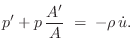
In terms of the logarithmic derivative of
Note that
Cylindrical Tubes
In the case of cylindrical tubes, the logarithmic derivative of the
area variation,
ln![]() , is zero, and Eq.
, is zero, and Eq.![]() (C.148)
reduces to the usual momentum conservation equation
(C.148)
reduces to the usual momentum conservation equation
![]() encountered when deriving the wave equation for plane waves
[318,349,47]. The present case reduces to the
cylindrical case when
encountered when deriving the wave equation for plane waves
[318,349,47]. The present case reduces to the
cylindrical case when

If we look at sinusoidal spatial waves,
![]() and
and
![]() , then
, then
![]() and
and
![]() , and the condition
for cylindrical-wave behavior becomes
, and the condition
for cylindrical-wave behavior becomes
![]() , i.e., the spatial
frequency of the wall variation must be much less than that of the
wave. Another way to say this is that the wall must be approximately
flat across a wavelength. This is true for smooth horns/bores at
sufficiently high wave frequencies.
, i.e., the spatial
frequency of the wall variation must be much less than that of the
wave. Another way to say this is that the wall must be approximately
flat across a wavelength. This is true for smooth horns/bores at
sufficiently high wave frequencies.
Wave Impedance in a Cone
From Eq.![]() (C.146) we have that the traveling-wave solution of the
wave equation in spherical coordinates can be expressed as
(C.146) we have that the traveling-wave solution of the
wave equation in spherical coordinates can be expressed as
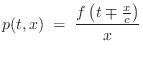
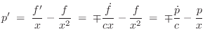
i.e., it can be expressed in terms of its own time derivative. This is a general property of any traveling wave.
![\includegraphics[width=\twidth]{eps/fconeparams}](http://www.dsprelated.com/josimages_new/pasp/img4294.png)
Referring to Fig.C.46, the area function ![]() can be
written for any cone in terms of the distance from its apex as
can be
written for any cone in terms of the distance from its apex as
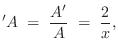
Substituting the logarithmic derivative of ![]() and
and ![]() from
Eq.
from
Eq.![]() (C.150) into the momentum-conservation equation
Eq. (C.148) yields
(C.150) into the momentum-conservation equation
Eq. (C.148) yields
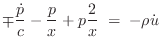
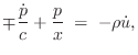
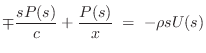
We can now solve for the wave impedance in each direction, where
the wave impedance may be defined (§7.1)
as the Laplace transform of the traveling pressure divided by
the Laplace transform of the corresponding traveling velocity wave:
 |
|||
 |
We introduce the shorthand
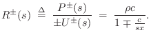
Note that for a cylindrical tube, the wave impedance in both directions is
![]() , and there is no frequency dependence. A wavelength
or more away from the conical tip, i.e., for
, and there is no frequency dependence. A wavelength
or more away from the conical tip, i.e., for
![]() ,
where
,
where ![]() is the spatial wavelength, the wave impedance again approaches
that of a cylindrical bore. However, in conical musical instruments,
the fundamental wavelength is typically twice the bore length, so the
complex nature of the wave impedance is important throughout the bore and
approaches being purely imaginary near the mouthpiece. This is
especially relevant to conical-bore double-reeds, such as the bassoon.
is the spatial wavelength, the wave impedance again approaches
that of a cylindrical bore. However, in conical musical instruments,
the fundamental wavelength is typically twice the bore length, so the
complex nature of the wave impedance is important throughout the bore and
approaches being purely imaginary near the mouthpiece. This is
especially relevant to conical-bore double-reeds, such as the bassoon.
Writing the wave impedance as
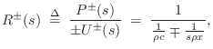
Up to now, we have been defining wave impedance as pressure divided by particle velocity. In acoustic tubes, volume velocity is what is conserved at a junction between two different acoustic tube types. Therefore, in acoustic tubes, we define the wave impedance as the ratio of pressure to volume velocity
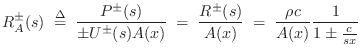
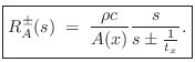
This is the wave impedance we use to compute the generalized reflection and transmission coefficients at a change in cross-sectional area and/or taper angle in a conical acoustic tube. Note that it has a zero at
In this case, the equivalent mass is
![]() . It would perhaps be more satisfying if the equivalent mass in
the conical wave impedance were instead
. It would perhaps be more satisfying if the equivalent mass in
the conical wave impedance were instead
![]() which is the
mass of air contained in a cylinder of radius
which is the
mass of air contained in a cylinder of radius ![]() projected back to
the tip of the cone. However, the ``acoustic mass'' cannot be
physically equivalent to mechanical mass. To see this, consider that
the impedance of a mechanical mass is
projected back to
the tip of the cone. However, the ``acoustic mass'' cannot be
physically equivalent to mechanical mass. To see this, consider that
the impedance of a mechanical mass is ![]() which is in physical units
of mass per unit time, and by definition of mechanical impedance this
equals force over velocity. The impedance in an acoustic tube, on the
other hand, must be in units of pressure (force/area) divided by
volume velocity (velocity
which is in physical units
of mass per unit time, and by definition of mechanical impedance this
equals force over velocity. The impedance in an acoustic tube, on the
other hand, must be in units of pressure (force/area) divided by
volume velocity (velocity ![]() area) and this reduces to
area) and this reduces to
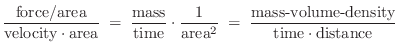
The real part of the wave impedance corresponds to transportation of wave
energy, the imaginary part is a so-called ``reactance'' and does not
correspond to power transfer. Instead, it corresponds to a ``standing
wave'' which is created by equal and opposite power flow, or an
``evanescent wave'' (§C.8.2), which is a non-propagating,
exponentially decaying, limiting form of a traveling wave in which the
``propagation constant'' is purely imaginary due to being at a
frequency above or below a ``cut off'' frequency for the waveguide
[295,122]. Driving an ideal mass at the end of a
waveguide results in total reflection of all incident wave energy
along with a quarter-cycle phase shift. Another interpretation is
that the traveling wave becomes a standing wave at the tip of the
cone. This is one way to see how the resonances of a cone can be the
same as those of a cylinder the same length which is open on
both ends. (One might first expect the cone to behave like a
cylinder which is open on one end and closed on the other.) Because
the impedance approaches a purely imaginary zero at the tip, it looks
like a mass (with impedance
![]() ). The ``piston of air'' at
the open end similarly looks like a mass
[285].
). The ``piston of air'' at
the open end similarly looks like a mass
[285].
More General One-Parameter Waves
The wave impedance derivation above made use of known properties of waves
in cones to arrive at the wave impedances in the two directions of travel
in cones. We now consider how this solution might be generalized to
arbitrary bore shapes. The momentum conservation equation is already
applicable to any wavefront area variation ![]() :
:
Defining the spatially instantaneous phase velocity as
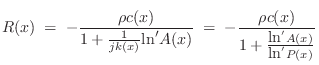
This reduces to the simple case of the uniform waveguide when the logarithmic derivative of cross-sectional area
Generalized Wave Impedance
Figure C.47 depicts a section of a conical bore which widens to the right connected to a section which narrows to the right. In addition, the cross-sectional areas are not matched at the junction.
The horizontal ![]() axis (taken along the boundary of the
cone) is chosen so that
axis (taken along the boundary of the
cone) is chosen so that ![]() corresponds to the apex of the cone. Let
corresponds to the apex of the cone. Let
![]() denote the cross-sectional area of the bore.
denote the cross-sectional area of the bore.
![\includegraphics[width=\twidth]{eps/fconecone}](http://www.dsprelated.com/josimages_new/pasp/img4350.png)
Since a piecewise-cylindrical approximation to a general acoustic tube can be regarded as a ``zeroth-order hold'' approximation. A piecewise conical approximation then uses first-order (linear) segments. One might expect that quadratic, cubic, etc., would give better and better approximations. However, such a power series expansion has a problem: In zero-order sections (cylinders), plane waves propagate as traveling waves. In first-order sections (conical sections), spherical waves propagate as traveling waves. However, there are no traveling wave types for higher-order waveguide flare (e.g., quadratic or higher) [357].
Since the digital waveguide model for a conic section is no more expensive to implement than that for a cylindrical section, (both are simply bidirectional delay lines), it would seem that modeling accuracy can be greatly improved for non-cylindrical bores (or parts of bores such as the bell) essentially for free. However, while the conic section itself costs nothing extra to implement, the scattering junctions between adjoining cone segments are more expensive computationally than those connecting cylindrical segments. However, the extra expense can be small. Instead of a single, real, reflection coefficient occurring at the interface between two cylinders of differing diameter, we obtain a first-order reflection filter at the interface between two cone sections of differing taper angle, as seen in the next section.
Generalized Scattering Coefficients
Generalizing the scattering coefficients at a multi-tube intersection
(§C.12) by replacing the usual real tube wave impedance
![]() by the complex generalized wave impedance
by the complex generalized wave impedance
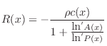
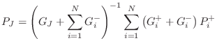
Cylinder with Conical Cap
Consider a cylindrical acoustic tube adjoined to a converging conical cap, as depicted in Figure C.48a. We may consider the cylinder to be either open or closed on the left side, but everywhere else it is closed. Since such a physical system is obviously passive, an interesting test of acoustic theory is to check whether theory predicts passivity in this case.
![\includegraphics[scale=0.9]{eps/cylconesp}](http://www.dsprelated.com/josimages_new/pasp/img4359.png) |
It is well known that a growing exponential appears at the junction of two conical waveguides when the waves in one conical taper angle reflect from a section with a smaller (or more negative) taper angle [7,300,8,160,9]. The most natural way to model a growing exponential in discrete time is to use an unstable one-pole filter [506]. Since unstable filters do not normally correspond to passive systems, we might at first expect passivity to not be predicted. However, it turns out that all unstable poles are ultimately canceled, and the model is stable after all, as we will see. Unfortunately, as is well known in the field of automatic control, it is not practical to attempt to cancel an unstable pole in a real system, even when it is digital. This is because round-off errors will grow exponentially in the unstable feedback loop and eventually dominate the output.
The need for an unstable filter to model reflection and transmission at a converging conical junction has precluded the use of a straightforward recursive filter model [406]. Using special ``truncated infinite impulse response'' (TIIR) digital filters [540], an unstable recursive filter model can in fact be used in practice [528]. All that is then required is that the infinite-precision system be passive, and this is what we will show in the special case of Fig.C.48.
Scattering Filters at the Cylinder-Cone Junction
As derived in §C.18.4, the wave impedance (for volume velocity)
at frequency ![]() rad/sec in a converging cone is given by
rad/sec in a converging cone is given by
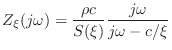 |
(C.152) |
where
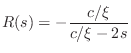
(where
The reflectance and transmittance from the right of the junction are the same when there is no wavefront area discontinuity at the junction [300]. Both
Reflectance of the Conical Cap
Let
![]() denote the time to propagate across the length of
the cone in one direction. As is well known [22], the reflectance
at the tip of an infinite cone is
denote the time to propagate across the length of
the cone in one direction. As is well known [22], the reflectance
at the tip of an infinite cone is ![]() for pressure waves. I.e., it
reflects like an open-ended cylinder. We ignore any absorption losses
propagating in the cone, so that the transfer function from the entrance of
the cone to the tip is
for pressure waves. I.e., it
reflects like an open-ended cylinder. We ignore any absorption losses
propagating in the cone, so that the transfer function from the entrance of
the cone to the tip is
![]() . Similarly, the transfer function from
the conical tip back to the entrance is also
. Similarly, the transfer function from
the conical tip back to the entrance is also
![]() . The complete
reflection transfer function from the entrance to the tip and back is then
. The complete
reflection transfer function from the entrance to the tip and back is then
| (C.155) |
Note that this is the reflectance a distance
We now want to interface the conical cap reflectance
![]() to the
cylinder. Since this entails a change in taper angle, there will be
reflection and transmission filtering at the cylinder-cone junction given
by Eq.
to the
cylinder. Since this entails a change in taper angle, there will be
reflection and transmission filtering at the cylinder-cone junction given
by Eq.![]() (C.154) and Eq.
(C.154) and Eq.![]() (C.155).
(C.155).
From inside the cylinder, immediately next to the cylinder-cone
junction shown in Fig.C.48, the reflectance of the conical cap is
readily derived from Fig.C.48b and Equations (C.154) and
(C.155) to be
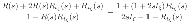 |
|||
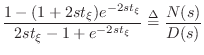 |
(C.156) |
where
| (C.157) |
is the numerator of the conical cap reflectance, and
| (C.158) |
is the denominator. Note that for very large
Stability Proof
A transfer function
![]() is stable if there are no poles in
the right-half
is stable if there are no poles in
the right-half ![]() plane. That is, for each zero
plane. That is, for each zero ![]() of
of ![]() , we must
have
re
, we must
have
re![]() . If this can be shown, along with
. If this can be shown, along with
![]() , then the reflectance
, then the reflectance ![]() is shown to be
passive. We must also study the system zeros (roots of
is shown to be
passive. We must also study the system zeros (roots of ![]() ) in order to
determine if there are any pole-zero cancellations (common factors in
) in order to
determine if there are any pole-zero cancellations (common factors in
![]() and
and ![]() ).
).
Since
re![]() if and only if
re
if and only if
re![]() , for
, for
![]() , we may set
, we may set
![]() without loss of generality. Thus, we need only
study the roots of
without loss of generality. Thus, we need only
study the roots of
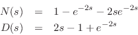
If this system is stable, we have stability also for all
![]() .
Since
.
Since ![]() is not a rational function of
is not a rational function of ![]() , the reflectance
, the reflectance ![]() may have infinitely many poles and zeros.
may have infinitely many poles and zeros.
Let's first consider the roots of the denominator
| (C.159) |
At any solution

To obtain separate equations for the real and imaginary parts, set
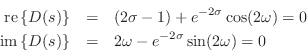
Both of these equations must hold at any pole of the reflectance. For
stability, we further require
![]() . Defining
. Defining
![]() and
and
![]() , we obtain the somewhat simpler conditions
, we obtain the somewhat simpler conditions
For any poles of ![]() on the
on the ![]() axis, we have
axis, we have ![]() , and
Eq.
, and
Eq.![]() (C.163) reduces to
(C.163) reduces to
It is well known that the ``sinc function''
We have so far proved that any poles on the ![]() axis must be at
axis must be at
![]() .
.
The same argument can be extended to the entire right-half
plane as follows. Going back to the more general case of
Eq.![]() (C.163), we have
(C.163), we have
 |
(C.164) |
Since
In the left-half plane, there are many potential poles.
Equation (C.162) has infinitely many solutions for each ![]() since the elementary inequality
since the elementary inequality
![]() implies
implies
![]() . Also, Eq.
. Also, Eq.![]() (C.163) has an increasing
number of solutions as
(C.163) has an increasing
number of solutions as ![]() grows more and more negative; in the limit of
grows more and more negative; in the limit of
![]() , the number of solutions is infinite and given by the roots
of
, the number of solutions is infinite and given by the roots
of ![]() (
(
![]() for any integer
for any integer ![]() ).
However, note that at
).
However, note that at
![]() , the solutions of Eq.
, the solutions of Eq.![]() (C.162) converge to the roots of
(C.162) converge to the roots of
![]() (
(
![]() for any integer
for any integer ![]() ).
The only issue is that the solutions of Eq.
).
The only issue is that the solutions of Eq.![]() (C.162) and Eq.
(C.162) and Eq.![]() (C.163)
must occur together.
(C.163)
must occur together.
![\includegraphics[width=3.5in]{eps/cylconelhp}](http://www.dsprelated.com/josimages_new/pasp/img4420.png) |
Figure C.49 plots the locus of real-part zeros (solutions to
Eq.![]() (C.162)) and imaginary-part zeros (Eq.
(C.162)) and imaginary-part zeros (Eq.![]() (C.163)) in a portion
the left-half plane. The roots at
(C.163)) in a portion
the left-half plane. The roots at ![]() can be seen at the
middle-right. Also, the asymptotic interlacing of these loci can be
seen along the left edge of the plot. It is clear that the two loci
must intersect at infinitely many points in the left-half plane near
the intersections indicated in the graph. As
can be seen at the
middle-right. Also, the asymptotic interlacing of these loci can be
seen along the left edge of the plot. It is clear that the two loci
must intersect at infinitely many points in the left-half plane near
the intersections indicated in the graph. As
![]() becomes
large, the intersections evidently converge to the peaks of the
imaginary-part root locus (a log-sinc function rotated
90 degrees). At all frequencies
becomes
large, the intersections evidently converge to the peaks of the
imaginary-part root locus (a log-sinc function rotated
90 degrees). At all frequencies ![]() , the roots occur near
the log-sinc peaks, getting closer to the peaks as
, the roots occur near
the log-sinc peaks, getting closer to the peaks as
![]() increases. The log-sinc peaks thus provide a reasonable estimate
number and distribution in the left-half
increases. The log-sinc peaks thus provide a reasonable estimate
number and distribution in the left-half ![]() -plane. An outline of an
analytic proof is as follows:
-plane. An outline of an
analytic proof is as follows:
- Rotate the loci in Fig.C.49 counterclockwise by 90 degrees.
- Prove that the two root loci are continuous, single-valued functions of
 (as the figure suggests).
- Prove that for
 , there are infinitely many extrema
of the log-sinc function (imaginary-part root-locus) which have
negative curvature and which lie below
, there are infinitely many extrema
of the log-sinc function (imaginary-part root-locus) which have
negative curvature and which lie below  (as the figure
suggests). The
(as the figure
suggests). The  and
and  lines are shown in the
figure as dotted lines.
lines are shown in the
figure as dotted lines.
- Prove that the other root locus (for the real part) has
infinitely many similar extrema which occur for
 (again as
the figure suggests).
(again as
the figure suggests).
- Prove that the two root-loci interlace at
 (already done above).
- Then topologically, the continuous functions must cross at
infinitely many points in order to achieve interlacing at
.
The peaks of the log-sinc function not only indicate approximately where the left-half-plane roots occur
Reflectance Magnitude
We have shown that the conical cap reflectance has no poles in the
strict right-half plane. For passivity, we also need to show that its
magnitude is bounded by unity for all ![]() on the
on the ![]() axis.
axis.
We have
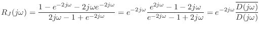
Poles at 
We know from the above that the denominator of the cone reflectance
has at least one root at ![]() . In this subsection we investigate
this ``dc behavior'' of the cone more thoroughly.
. In this subsection we investigate
this ``dc behavior'' of the cone more thoroughly.
A hasty analysis based on the reflection and transmission filters in
Equations (C.154) and (C.155) might conclude that the reflectance
of the conical cap converges to ![]() at dc, since
at dc, since ![]() and
and ![]() .
However, this would be incorrect. Instead, it is necessary to take the
limit as
.
However, this would be incorrect. Instead, it is necessary to take the
limit as
![]() of the complete conical cap reflectance
of the complete conical cap reflectance ![]() :
:
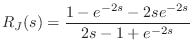 |
(C.165) |
We already discovered a root at
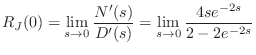 |
(C.166) |
and once again the limit is an indeterminate
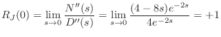 |
(C.167) |
Thus, two poles and zeros cancel at dc, and the dc reflectance is
Another method of showing this result is to form a Taylor series expansion
of the numerator and denominator:
 |
(C.168) | ||
 |
(C.169) |
Both series begin with the term
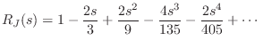 |
(C.170) |
which approaches
An alternative analysis of this issue is given by Benade in [37].
Next Section:
Finite-Difference Schemes
Previous Section:
Elementary Physics, Mechanics, and Acoustics


