


Digital Waveguides
A (lossless) digital waveguide is defined as a
bidirectional delay line at some wave impedance ![]() [430,433].
Figure 2.11 illustrates one digital waveguide.
[430,433].
Figure 2.11 illustrates one digital waveguide.

As before, each delay line contains a sampled acoustic traveling wave.
However, since we now have a bidirectional delay line, we have
two traveling waves, one to the ``left'' and one to the
``right'', say. It has been known since 1747 [100] that
the vibration of an ideal string
can be described as the sum of two traveling waves going in opposite
directions. (See Appendix C for a mathematical derivation of this
important fact.) Thus, while a single delay line can model an
acoustic plane wave, a bidirectional delay line (a digital
waveguide) can model any one-dimensional linear acoustic system such
as a violin string, clarinet bore, flute pipe, trumpet-valve pipe, or
the like. Of course, in real acoustic strings and bores, the 1D
waveguides exhibit some loss and
dispersion3.4 so that we will need some filtering in
the waveguide to obtain an accurate physical model of such systems.
The wave impedance ![]() (derived in Chapter 6) is
needed for connecting digital waveguides to other physical simulations
(such as another digital waveguide or finite-difference model).
(derived in Chapter 6) is
needed for connecting digital waveguides to other physical simulations
(such as another digital waveguide or finite-difference model).
Physical Outputs
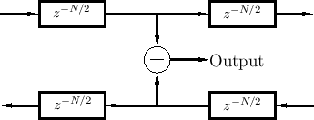
Physical variables (force, pressure, velocity, ...) are obtained by summing traveling-wave components, as shown in Fig.2.12, and more elaborated in Fig.2.13.
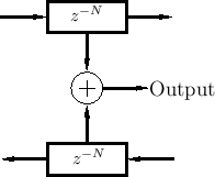
It is important to understand that the two traveling waves in a digital waveguide are now components of a more general acoustic vibration. The physical wave vibration is obtained by summing the left- and right-going traveling waves. A traveling wave by itself in one of the delay lines is no longer regarded as ``physical'' unless the signal in the opposite-going delay line is zero. Traveling waves are efficient for simulation, but they are not easily estimated from real-world measurements [476], except when the traveling-wave component in one direction can be arranged to be zero.
Note that traveling-wave components are not necessarily unique. For example, we can add a constant to the right-going wave and subtract the same constant from the left-going wave without altering the (physical) sum [263]. However, as derived in Appendix C (§C.3.6), 1D traveling-wave components are uniquely specified by two linearly independent physical variables along the waveguide, such as position and velocity (vibrating strings) or pressure and velocity (acoustic tubes).
Physical Inputs
A digital waveguide input signal corresponds to a disturbance of the 1D propagation medium. For example, a vibrating string is plucked or bowed by such an external disturbance. The result of the disturbance is wave propagation to the left and right of the input point. By physical symmetry, the amplitude of the left- and right-going propagating disturbances will normally be equal.3.5 If the disturbance superimposes with the waves already passing through at that point (an idealized case), then it is purely an additive input, as shown in Fig.2.14.
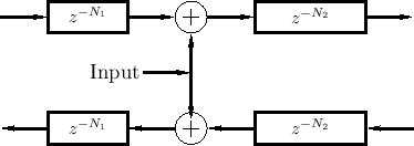 |
Note that the superimposing input of Fig.2.14 is the graph-theoretic transpose of the ideal output shown in Fig.2.13. In other words, the superimposing input injects by means of two transposed taps. Transposed taps are discussed further in §2.5.2 below.
In practical reality, physical driving inputs do not merely superimpose with the current state of the driven system. Instead, there is normally some amount of interaction with the current system state (when it is nonzero), as discussed further in the next section. Note that there are similarly no ideal outputs as depicted in Fig.2.13. Real physical ouputs must present some kind of load on the system (energy must be extracted). Superimposing inputs and non-loading outputs are ideals that are often approximated in real-world systems. Of course, in the virtual world, they are no problem at all--in fact, they are usually easier to implement, and more efficient.
Interacting Physical Input
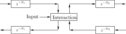
Figure 2.15 shows the general case of an input signal that interacts with the state of the system at one point along the waveguide. Since the interaction is physical, it only depends on the ``incoming state'' (traveling-wave components) and the driving input signal.
 |
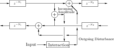
A less general but commonly encountered case is shown in Fig.2.16. This case requires the ``outgoing disturbance'' to be distributed equally to the left and right, and it sums with the incoming waves to produce the outgoing waves.
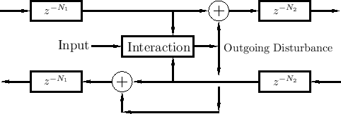
Figure 2.17 shows a further reduction in generality--also commonly encountered--in which the interaction depends only on the amplitude of the simulated physical variable (such as string velocity or displacement). The incoming amplitude is formed as the sum of the incoming traveling-wave components. We will encounter examples of this nature in later chapters (such as Chapter 9). It provides realistic models of physical excitations such as a guitar plectra, violin bows, and woodwind reeds.
 |
If an output signal is desired at this precise point, it can be computed as the incoming amplitude plus twice the outgoing disturbance signal (equivalent to summing the inputs of the two outgoing delay lines).
Note that the above examples all involve waveguide excitation at a single spatial point. While this can give a sufficiently good approximation to physical reality in many applications, one should also consider excitations that are spread out over multiple spatial samples (even just two).
We will develop the topic of digital waveguide modeling more systematically in Chapter 6 and Appendix C, among other places in this book. This section is intended only as a high-level preview and overview. For the next several chapters, we will restrict attention to normal signal processing structures in which signals may have physical units (such as acoustic pressure), and delay lines hold sampled acoustic waves propagating in one direction, but successive processing blocks do not ``load each other down'' or connect ``bidirectionally'' (as every truly physical interaction must, by Newton's third law3.6). Thus, when one processing block feeds a signal to a next block, an ``ideal output'' drives an ``ideal input''. This is typical in digital signal processing: Loading effects and return waves3.7 are neglected.3.8
Next Section:
Tapped Delay Line (TDL)
Previous Section:
Lossy Acoustic Propagation


