


Doppler Simulation
It is well known that a time-varying delay line results in a frequency shift. Time-varying delay is often used, for example, to provide vibrato and chorus effects [17]. We therefore expect a time-varying delay-line to be capable of precise Doppler simulation. This section discusses simulating the Doppler effect using a variable delay line [468].6.6
Consider Doppler shift from a physical point of view. The air can be
considered as analogous to a magnetic tape which moves from
source to listener at speed ![]() (see Fig.5.4). The source is
analogous to the
write-head of a tape recorder, and the listener corresponds to the
read-head. When the source and listener are fixed, the listener
receives what the source records. When either moves, a Doppler shift
is observed by the listener, according
to Eq.
(see Fig.5.4). The source is
analogous to the
write-head of a tape recorder, and the listener corresponds to the
read-head. When the source and listener are fixed, the listener
receives what the source records. When either moves, a Doppler shift
is observed by the listener, according
to Eq.![]() (5.2).6.7
(5.2).6.7

Doppler Simulation via Delay Lines
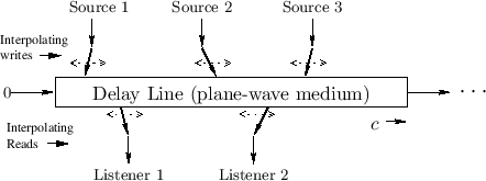
This analogy also works for a delay-line based computational model,
as depicted in Fig.5.5.
The magnetic tape is now the delay line, the tape read-head is the
read-pointer of the delay line, and the write-head is the delay-line
write-pointer. In this analogy, it is readily verified
that modulating delay by changing the read-pointer increment from 1 to
![]() (thereby requiring interpolated reads) corresponds to
listener motion away from the source at speed
(thereby requiring interpolated reads) corresponds to
listener motion away from the source at speed ![]() . It also follows
that changing the write-pointer increment from
. It also follows
that changing the write-pointer increment from ![]() to
to
![]() corresponds source motion toward the listener at
speed
corresponds source motion toward the listener at
speed ![]() .
When this is done, we must use interpolating writes into the
delay memory. Interpolating writes may be called
de-interpolation [502], and they are formally the
graph-theoretic transpose of interpolating reads (ordinary
``interpolation'') [333]. A review of
time-varying, interpolating, delay-line reads and writes, together
with a method using a single shared pointer, are given in
[383].
.
When this is done, we must use interpolating writes into the
delay memory. Interpolating writes may be called
de-interpolation [502], and they are formally the
graph-theoretic transpose of interpolating reads (ordinary
``interpolation'') [333]. A review of
time-varying, interpolating, delay-line reads and writes, together
with a method using a single shared pointer, are given in
[383].
Time-Varying Delay-Line Reads
If ![]() denotes the input to a time-varying delay, the output can be
written as
denotes the input to a time-varying delay, the output can be
written as
Let's analyze the frequency shift caused by a time-varying delay by
setting ![]() to a complex sinusoid at frequency
to a complex sinusoid at frequency ![]() :
:
where
Comparing Eq.![]() (5.6) to Eq.
(5.6) to Eq.![]() (5.2), we find that the
time-varying delay most naturally simulates Doppler shift caused by a
moving listener, with
(5.2), we find that the
time-varying delay most naturally simulates Doppler shift caused by a
moving listener, with
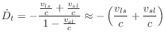
That is, the delay growth-rate,
Simulating source motion is also possible, but the relation
between delay change and desired frequency shift is more complex, viz.,
from Eq.![]() (5.2) and Eq.
(5.2) and Eq.![]() (5.6),
(5.6),
The time-varying delay line was described in §5.1. As discussed there, to implement a continuously varying delay, we add a ``delay growth parameter'' g to the delayline function in Fig.5.1, and change the line
rptr += 1; // pointer updateto
rptr += 1 - g; // pointer updateWhen g is 0, we have a fixed delay line, corresponding to
Note that when the read- and write-pointers are driven directly from a model of physical propagation-path geometry, they are always separated by predictable minimum and maximum delay intervals. This implies it is unnecessary to worry about the read-pointer passing the write-pointers or vice versa. In generic frequency shifters [275], or in a Doppler simulator not driven by a changing geometry, a pointer cross-fade scheme may be necessary when the read- and write-pointers get too close to each other.
Multiple Read Pointers
Using multiple read pointers, multiple listeners can be simulated. Furthermore, each read-pointer signal can be filtered to simulate propagation losses and radiation characteristics of the source in the direction of the listener. The read-pointers can move independently to simulate the different Doppler shifts associated with different listener motions and relative source directions.
Multiple Write Pointers
It is interesting to consider also what effects can be achieved using multiple interpolating write pointers. From the considerations in §5.7.1, we see that multiple write-pointers correspond to multiple write-heads on a magnetic tape recorder. If they are arranged at a fixed spacing, they are equivalent to multiple read pointers, providing a basic multipath simulation. If, however, the write pointers are moving independently, they induce independent Doppler shifts due to source motion. In particular, each write-pointer can lay down a signal from a separate source to a single listener with its own Doppler shift. Furthermore, each write-signal can be passed through its own filter. Such an individualized source filter can implement all filtering incurred along the propagation path from each source to the listener.
When all write pointers have the same input signal, their filters can be implemented using a series chain in which the outputs of successive filters in the chain correspond to progressively longer propagation paths (progressively more filtering). Such an implementation can greatly reduce the filter order required for propagation paths longer than the shortest.
The write-pointers may cross each other with no ill effects, since all but the first6.8 simply sum into the shared delay line.
We have seen that a single delay line can be used to simulate any
number of moving listeners (§5.7.3) or any number of moving
sources. However, when simulating both multiple listeners and
multiple sources, it is not possible to share a single delay line.
This is because the different listeners do not see the same Doppler
shift for each moving source, and while the listener's read-pointer
motion can be adjusted to correct for the Doppler shift seen from any
particular source, it cannot correct for more than one in general.
Thus, in general, we need as many delay lines as there are sources or
listeners, whichever is smaller. More precisely, if there are ![]() moving sources and
moving sources and ![]() moving listeners, simulation requires
moving listeners, simulation requires
![]() delay lines.
delay lines.
Stereo Processing
As a special case, stereo processing of any number of sources can be accomplished using two delay lines, corresponding to left and right stereo channels. The stereo mix may contain a panned mixture of any number sources, each with its own stereo placement, path filtering, and Doppler shift. The two stereo outputs may correspond to ``left and right ears,'' or, more generally, to left- and right-channel microphones in a studio recording set-up.
System Block Diagram
A schematic diagram of a stereo multiple-source simulation is shown in Fig.5.6. To simplify the layout, the input and output signals are all on the right in the diagram. For further simplicity, only one input source is shown. Additional input sources are handled identically, summing into the same delay lines in the same way.
![\includegraphics[width=0.8\twidth]{eps/bdiag}](http://www.dsprelated.com/josimages_new/pasp/img1284.png) |
The input source signal first passes through filter ![]() , which
provides time-invariant filtering common to all propagation
paths. The left- and right-channel filters
, which
provides time-invariant filtering common to all propagation
paths. The left- and right-channel filters
![]() and
and
![]() are typically low-order, linear, time-varying
filters implementing the time-varying characteristics of the shortest
(time-varying) propagation path from the source to each listener.
(The
are typically low-order, linear, time-varying
filters implementing the time-varying characteristics of the shortest
(time-varying) propagation path from the source to each listener.
(The ![]() superscript here indicates a time-varying filter.) These
filter outputs sum into the delay lines at arbitrary
(time-varying) locations using interpolating writes.
The zero signals entering each delay line on the
left can be omitted if the left-most filter overwrites delay memory
instead of summing into it.
superscript here indicates a time-varying filter.) These
filter outputs sum into the delay lines at arbitrary
(time-varying) locations using interpolating writes.
The zero signals entering each delay line on the
left can be omitted if the left-most filter overwrites delay memory
instead of summing into it.
The outputs of
![]() and
and
![]() in Fig.5.6
correspond to the ``direct signal'' from the moving source, when a
direct signal exists. These filters may incorporate modulation of
losses due to the changing propagation distance from the moving source
to each listener, and they may include dynamic equalization
corresponding to the changing radiation strength in different
directions from the moving (and possibly turning) source toward each
listener.
in Fig.5.6
correspond to the ``direct signal'' from the moving source, when a
direct signal exists. These filters may incorporate modulation of
losses due to the changing propagation distance from the moving source
to each listener, and they may include dynamic equalization
corresponding to the changing radiation strength in different
directions from the moving (and possibly turning) source toward each
listener.
The next trio of filters in Fig.5.6, ![]() ,
,
![]() ,
and
,
and
![]() , correspond to the next-to-shortest acoustic propagation
path, typically the ``first reflection,'' such as from a wall close to
the source. Since a reflection path is longer than the direct path, and since a reflection
itself can attenuate (or scatter) an incident sound ray, there is
generally more filtering required relative to the direct signal. This
additional filtering can be decomposed into its fixed component
, correspond to the next-to-shortest acoustic propagation
path, typically the ``first reflection,'' such as from a wall close to
the source. Since a reflection path is longer than the direct path, and since a reflection
itself can attenuate (or scatter) an incident sound ray, there is
generally more filtering required relative to the direct signal. This
additional filtering can be decomposed into its fixed component
![]() and time-varying components
and time-varying components
![]() and
and
![]() .
.
Note that acceptable results may be obtained without implementing all
of the filters indicated in Fig.5.6. Furthermore, it can be
convenient to incorporate ![]() into
into
![]() and
and
![]() when doing so does not increase their orders
significantly.
when doing so does not increase their orders
significantly.
Note also that the source-filters
![]() and
and
![]() may include HRTF filtering [57,545]
in order to impart illusory angles of arrival in 3D space.
may include HRTF filtering [57,545]
in order to impart illusory angles of arrival in 3D space.
Next Section:
Chorus Effect
Previous Section:
Doppler Effect


