Sign in

Search Online Books

Free Online Books

Sponsor

Industry's highest performing at the lowest power DSPs now as low as $5.00*
Start development today!
*volume pricing for 10ku

Chapters

Physical Audio Signal Processing
    Digital Waveguide Models
       Loop Filter Identification
          EDR-Based Loop-Filter Design

Chapter Contents:

Search Physical Audio Signal Processing

Book Index | Global Index

Would you like to be notified by email when Julius Orion Smith III publishes a new entry into his blog?

EDR-Based Loop-Filter Design

This section discusses use of the Energy Decay Relief (EDR) (§3.2.2) to measure the decay times of the partial overtones in a recorded vibrating string.

First we derive what to expect in the case of a simplified string model along the lines discussed in §6.7 above. Assume we have the synthesis model of Fig.6.12, where now the loss factor is replaced by the digital filter that we wish to design. Let $\underline{x}(n)$ denote the contents of the delay line as a vector at time , with $\underline{x}(0)$ denoting the initial contents of the delay line.

For simplicity, we define the EDR based on a length DFT of the delay-line vector $\underline{x}$ , and use a rectangular window with a ``hop size'' of samples, i.e.,

$\displaystyle \underline{X}_m(\omega_k) \isdef \dft _{N,\omega_k}\{\underline{x}_m\}, \quad m=0,1,2,\ldots,$

where $\underline{x}_m(n)\isdef \underline{x}(mN)$ . That is $\underline{x}_m$ is simply the

th successive snapshot of the delay-line contents, where the snapshots are taken once every

samples. We may interpret $\underline{X}_m$ as

th short-time spectrum of the output signal $y^{+}(n)$ shown in Fig.6.12. Due to the special structure of our synthesis model, we have

$\displaystyle \underline{X}_m(\omega_k) = H_l^m(\omega_k) \underline{X}_0(\omega_k)$

for each DFT bin number $k\in[0,N-1]$ .

Applying the definition of the EDR (§3.2.2) to this short-time spectrum gives

$\begin{eqnarray*} E_m(\omega_k) &\isdef & \sum_{\nu=m}^\infty \left\vert\underl... ...omega_k)\right\vert^2} \left\vert H_l(\omega_k)\right\vert^{2m}. \end{eqnarray*}$

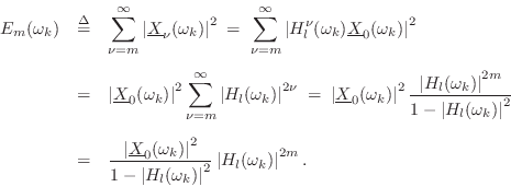
We therefore have the following recursion for successive EDR time-slices:^7.13

$\displaystyle E_{m+1}(\omega_k) = \left\vert H_l(\omega_k)\right\vert^2 E_m(\omega_k)$

Since we normally try to fit straight-line decays to the EDR on a log scale (typically a decibel scale), we will see the relation

$\displaystyle \log(E_{m+1}) = \log(E_m) + \log(\vert H_l\vert^2),$

where the common argument $\omega_k$ is dropped for notational simplicity. Since we require $\vert H_l(\omega_k)\vert<1$ for stability of the filtered-delay loop, the EDR decays monotonically in this example. Thus, the measured slope of the partial overtone decays will be found to be proportional to $\log(\vert H_l\vert)$ .

This analysis can be generalized to a time-varying model in which the loop filter is allowed to change once per ``period'' .^7.14

An online laboratory exercise covering the practical details of measuring overtone decay-times and designing a corresponding loop filter is given in [280].

Previous: Extension to Stiff Strings
Next: String Coupling Effects

Order a Hardcopy of Physical Audio Signal Processing

About the Author: Julius Orion Smith III
Julius Smith's background is in electrical engineering (BS Rice 1975, PhD Stanford 1983). He is presently Professor of Music and Associate Professor (by courtesy) of Electrical Engineering at Stanford's Center for Computer Research in Music and Acoustics (CCRMA), teaching courses and pursuing research related to signal processing applied to music and audio systems. See http://ccrma.stanford.edu/~jos/ for details.

Comments

No comments yet for this page

Add a Comment

You need to login before you can post a comment (best way to prevent spam). ( Not a member? )