


Elementary Physics, Mechanics, and Acoustics
This appendix derives some basic results from the field of physics, particularly mechanics and acoustics, which are referenced elsewhere in this book, or which are known to be needed in practical synthesis models.
Newton's Laws of Motion
Perhaps the most heavily used equation in physics is Newton's second law of motion:
In this formulation, the applied force
Newton's Three Laws of Motion
Newton's three laws of motion may be stated as follows:
- Every object in a state of uniform motion will remain in that
state of motion unless an external force acts on it.
- Force equals mass times acceleration [
 ].
].
- For every action there is an equal and opposite reaction.
The first law, also called the law of inertia, was pioneered by Galileo. This was quite a conceptual leap because it was not possible in Galileo's time to observe a moving object without at least some frictional forces dragging against the motion. In fact, for over a thousand years before Galileo, educated individuals believed Aristotle's formulation that, wherever there is motion, there is an external force producing that motion.
The second law,
![]() , actually implies the first law, since
when
, actually implies the first law, since
when ![]() (no applied force), the acceleration
(no applied force), the acceleration ![]() is zero,
implying a constant velocity
is zero,
implying a constant velocity ![]() . (The velocity is simply the
integral with respect to time of
. (The velocity is simply the
integral with respect to time of
![]() .)
.)
Newton's third law implies conservation of momentum [137]. It can also be seen as following from the second law: When one object ``pushes'' a second object at some (massless) point of contact using an applied force, there must be an equal and opposite force from the second object that cancels the applied force. Otherwise, there would be a nonzero net force on a massless point which, by the second law, would accelerate the point of contact by an infinite amount.
In summary, Newton's laws boil down to ![]() . An enormous quantity
of physical science has been developed by applying this
simpleB.1 mathematical law to different physical
situations.
. An enormous quantity
of physical science has been developed by applying this
simpleB.1 mathematical law to different physical
situations.
Mass
Mass is an intrinsic property of matter.
From Newton's second law,
![]() , we have that the amount of
force required to accelerate an object, by a given amount, is
proportional to its mass. Thus, the mass of an object quantifies its
inertia--its resistance to a change in velocity.
, we have that the amount of
force required to accelerate an object, by a given amount, is
proportional to its mass. Thus, the mass of an object quantifies its
inertia--its resistance to a change in velocity.
We can measure the mass of an object by measuring the
gravitational force between it and another known mass,
as described in the next section. This is a special case of measuring
its acceleration in response to a known force. Whatever the force ![]() ,
the mass
,
the mass ![]() is given by
is given by ![]() divided by the resulting acceleration
divided by the resulting acceleration
![]() , again by Newton's second law
, again by Newton's second law ![]() .
.
The usual mathematical model for an ideal mass is a dimensionless point at some location in space. While no real objects are dimensionless, they can often be treated mathematically as dimensionless points located at their center of mass, or centroid (§B.4.1).
The physical state of a mass ![]() at time
at time ![]() consists of its
position
consists of its
position ![]() and velocity
and velocity
![]() in 3D space.
The amount of mass itself,
in 3D space.
The amount of mass itself, ![]() , is regarded as a fixed parameter that
does not change. In other words, the state
, is regarded as a fixed parameter that
does not change. In other words, the state
![]() of a
physical system typically changes over time, while any
parameters of the system, such as mass
of a
physical system typically changes over time, while any
parameters of the system, such as mass ![]() , remain fixed over
time (unless otherwise specified).
, remain fixed over
time (unless otherwise specified).
Gravitational Force
We are all familiar with the force of gravity. It is a
fundamental observed property of our universe that any two masses
![]() and
and ![]() experience an attracting force
experience an attracting force ![]() given by the
formula
given by the
formula
where
The law of gravitation Eq.![]() (B.2) can be accepted as an
experimental fact which defines the concept of a force.B.3 The giant conceptual leap taken by Newton was that the law of
gravitation is
universal--applying to celestial bodies as well as objects on
earth. When a mass is ``dropped'' and allowed to ``fall'' in a
gravitational field, it is observed to experience a
uniform acceleration proportional to its mass. Newton's second
law of motion (§B.1) quantifies this result.
(B.2) can be accepted as an
experimental fact which defines the concept of a force.B.3 The giant conceptual leap taken by Newton was that the law of
gravitation is
universal--applying to celestial bodies as well as objects on
earth. When a mass is ``dropped'' and allowed to ``fall'' in a
gravitational field, it is observed to experience a
uniform acceleration proportional to its mass. Newton's second
law of motion (§B.1) quantifies this result.
Hooke's Law
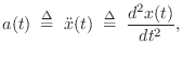
Consider an ideal spring suspending a mass from a rigid ceiling, as
depicted in Fig.B.1. Assume the mass is at rest,
and that its distance ![]() from the ceiling is fixed.
from the ceiling is fixed.
If ![]() denotes the mass of the earth, and
denotes the mass of the earth, and ![]() is the distance of mass
is the distance of mass
![]() 's center from the earth's center of mass, then the downward force
on the mass
's center from the earth's center of mass, then the downward force
on the mass ![]() is given by Eq.
is given by Eq.![]() (B.2) as
(B.2) as

where
Note that the force on the spring in Fig.B.1 is gravitational force. Equal and opposite to the force of gravity is the spring force exerted upward by the spring on the mass (which is not moving). We know that the spring force is equal and opposite to the gravitational force because the mass would otherwise be accelerated by the net force.B.4 Therefore, like gravity, a displaced spring can be regarded as a definition of an applied force. That is, whenever you have to think of an applied force, you can always consider it as being delivered by the end of some ideal spring attached to some external physical system.
Note, by the way, that normal interaction forces when objects touch arise from the Coulomb force (electrostatic force, or repulsion of like charges) between electron orbitals. This electrostatic force obeys an ``inverse square law'' like gravity, and therefore also behaves like an ideal spring for small displacements.B.5
The specific value of ![]() depends on the physical units adopted as
well as the ``stiffness'' of the spring. What is most important in
this definition of force is that a doubling of spring displacement
doubles the force. That is, the spring force is a linear
function of spring displacement (compression or stretching).
depends on the physical units adopted as
well as the ``stiffness'' of the spring. What is most important in
this definition of force is that a doubling of spring displacement
doubles the force. That is, the spring force is a linear
function of spring displacement (compression or stretching).
Applying Newton's Laws of Motion
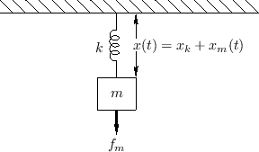
As a simple example, consider a mass ![]() driven along a frictionless
surface by an ideal spring
driven along a frictionless
surface by an ideal spring ![]() , as shown in Fig.B.2.
Assume that the mass position
, as shown in Fig.B.2.
Assume that the mass position ![]() corresponds to the spring at rest,
i.e., not stretched or compressed. The force necessary to compress the
spring by a distance
corresponds to the spring at rest,
i.e., not stretched or compressed. The force necessary to compress the
spring by a distance ![]() is given by Hooke's law (§B.1.3):
is given by Hooke's law (§B.1.3):
where we have defined
where
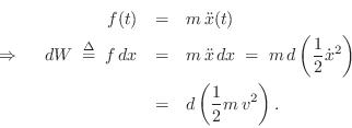
Work = Force times Distance = Energy
Work is defined as force times distance. Work is a measure of the energy expended in applying a force to move an object.B.8
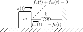
The work required to compress a spring ![]() through a displacement of
through a displacement of ![]() meters, starting from rest, is then
meters, starting from rest, is then
Work can also be negative. For example, when uncompressing an ideal spring, the (positive) work done by the spring on its moving end support can be interpreted also as saying that the end support performs negative work on the spring as it allows the spring to uncompress. When negative work is performed, the driving system is always accepting energy from the driven system. This is all simply accounting. Physically, one normally considers the driver as the agent performing the positive work, i.e., the one expending energy to move the driven object. Thus, when allowing a spring to uncompress, we consider the spring as performing (positive) work on whatever is attached to its moving end.
During a sinusoidal mass-spring oscillation, as derived in §B.1.4, each period of the oscillation can be divided into equal sections during which either the mass performs work on the spring, or vice versa.
Gravity, spring forces, and electrostatic forces are examples of
conservative forces. Conservative forces have the property
that the work required to move an object from point ![]() to point
to point ![]() ,
either with or against the force, depends only on the locations of
points
,
either with or against the force, depends only on the locations of
points ![]() and
and ![]() in space, not on the path taken from
in space, not on the path taken from ![]() to
to ![]() .
.
Potential Energy in a Spring
When compressing an ideal spring, work is performed, and this
work is stored in the spring in the form of what we call
potential energy. Equation (B.6) above gives the quantitative
formula for the potential energy ![]() stored in an ideal spring
after it has been compressed
stored in an ideal spring
after it has been compressed ![]() meters from rest.
meters from rest.
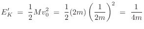
Kinetic Energy of a Mass
Kinetic energy is energy associated with motion. For example, when a spring uncompresses and accelerates a mass, as in the configuration of Fig.B.2, work is performed on the mass by the spring, and we say that the potential energy of the spring is converted to kinetic energy of the mass.
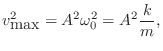
Suppose in Fig.B.2 we have an initial spring compression
by ![]() meters at time
meters at time ![]() , and the mass velocity is zero at
, and the mass velocity is zero at
![]() . Then from the equation of motion Eq.
. Then from the equation of motion Eq.![]() (B.5), we can calculate
when the spring returns to rest (
(B.5), we can calculate
when the spring returns to rest (![]() ). This first happens at the
first zero of
). This first happens at the
first zero of
![]() , which is time
, which is time
![]() . At this time, the velocity,
given by the time-derivative of Eq.
. At this time, the velocity,
given by the time-derivative of Eq.![]() (B.5),
(B.5),
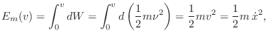
Mass Kinetic Energy from Virtual Work
From Newton's second law,
![]() (introduced in Eq.
(introduced in Eq.![]() (B.1)),
we can use d'Alembert's idea of virtual work to derive the
formula for the kinetic energy of a mass given its speed
(B.1)),
we can use d'Alembert's idea of virtual work to derive the
formula for the kinetic energy of a mass given its speed
![]() .
Let
.
Let ![]() denote a small (infinitesimal) displacement of the mass in
the
denote a small (infinitesimal) displacement of the mass in
the ![]() direction. Then we have, using the calculus of differentials,
direction. Then we have, using the calculus of differentials,
Thus, by Newton's second law, a differential of work ![]() applied to a
mass
applied to a
mass ![]() by force
by force ![]() through distance
through distance ![]() boosts the kinetic energy
of the mass by
boosts the kinetic energy
of the mass by
![]() . The kinetic energy of a mass moving at
speed
. The kinetic energy of a mass moving at
speed ![]() is then given by the integral of all such differential
boosts from 0 to
is then given by the integral of all such differential
boosts from 0 to ![]() :
:
The quantity ![]() is classically called the virtual work
associated with force
is classically called the virtual work
associated with force ![]() , and
, and ![]() a virtual displacement
[544].
a virtual displacement
[544].
Energy in the Mass-Spring Oscillator
Summarizing the previous sections, we say that a compressed spring holds a potential energy equal to the work required to compress the spring from rest to its current displacement. If a compressed spring is allowed to expand by pushing a mass, as in the system of Fig.B.2, the potential energy in the spring is converted to kinetic energy in the moving mass.
We can draw some inferences from the oscillatory motion of the
mass-spring system written in Eq.![]() (B.5):
(B.5):
- From a global point of view, we see that energy is conserved, since the oscillation never decays.
- At the peaks of the displacement
 (when
(when
 is either
 or
or  ), all energy is in the form of potential energy,
i.e., the spring is either maximally compressed or stretched, and the mass
is momentarily stopped as it is changing direction.
), all energy is in the form of potential energy,
i.e., the spring is either maximally compressed or stretched, and the mass
is momentarily stopped as it is changing direction.
- At the zero-crossings of , the spring is momentarily
relaxed, thereby holding no potential energy; at these instants, all
energy is in the form of kinetic energy, stored in the motion of the mass.
- Since total energy is conserved (§B.2.5), the kinetic
energy of the mass at the displacement zero-crossings is exactly the
amount needed to stretch the spring to displacement
 (or compress
it to
(or compress
it to  ) before the mass stops and changes direction. At all
times, the total energy
) before the mass stops and changes direction. At all
times, the total energy  is equal to the sum of the potential
energy
is equal to the sum of the potential
energy  stored in the spring, and the kinetic energy
  stored in the mass:
![$\displaystyle \mbox{constant [$E_k(0)$]}$](http://www.dsprelated.com/josimages_new/pasp/img2672.png)
Energy Conservation
It is a remarkable property of our universe that energy is conserved under all circumstances. There are no known exceptions to the conservation of energy, even when relativistic and quantum effects are considered.B.9
Energy may be defined as the ability to do work, where work may be defined as force times distance (§B.2).
Energy Conservation in the Mass-Spring System
Recall that Newton's second law applied to a mass-spring system, as in §B.1.4, yields
![\begin{eqnarray*}
0
&=& m{\ddot x}(t){\dot x}(t) + k\,x(t){\dot x}(t)\\
&=& m\...
...{d}{dt} \left[ E_m(t) + E_k(t) \right]\\
&=& \frac{d}{dt} E(t).
\end{eqnarray*}](http://www.dsprelated.com/josimages_new/pasp/img2682.png)
Thus, Newton's second law and Hooke's law imply conservation of energy in the mass-spring system of Fig.B.2.
Momentum
The momentum of a mass ![]() is usually defined by
is usually defined by
Conservation of Momentum
Like energy, momentum is conserved in physical systems. For example, when two masses collide and recoil from each other, the total momentum after the collision equals that before the collision. Since the momentum is a three-dimensional vector in Euclidean space, momentum conservation provides three simultaneous equations, in general.B.10
Rigid-Body Dynamics
Below are selected topics from rigid-body dynamics, a subtopic of classical mechanics involving the use of Newton's laws of motion to solve for the motion of rigid bodies moving in 1D, 2D, or 3D space.B.11 We may think of a rigid body as a distributed mass, that is, a mass that has length, area, and/or volume rather than occupying only a single point in space. Rigid body models have application in stiff strings (modeling them as disks of mass interconnect by ideal springs), rigid bridges, resonator braces, and so on.
We have already used Newton's ![]() to formulate mathematical dynamic
models for the ideal point-mass (§B.1.1), spring
(§B.1.3), and a simple mass-spring system (§B.1.4).
Since many physical systems can be modeled as assemblies of masses and
(normally damped) springs, we are pretty far along already. However,
when the springs interconnecting our point-masses are very stiff, we
may approximate them as rigid to simplify our simulations. Thus,
rigid bodies can be considered mass-spring systems in which the
springs are so stiff that they can be treated as rigid massless rods
(infinite spring-constants
to formulate mathematical dynamic
models for the ideal point-mass (§B.1.1), spring
(§B.1.3), and a simple mass-spring system (§B.1.4).
Since many physical systems can be modeled as assemblies of masses and
(normally damped) springs, we are pretty far along already. However,
when the springs interconnecting our point-masses are very stiff, we
may approximate them as rigid to simplify our simulations. Thus,
rigid bodies can be considered mass-spring systems in which the
springs are so stiff that they can be treated as rigid massless rods
(infinite spring-constants ![]() , in the notation of §B.1.3).
, in the notation of §B.1.3).
So, what is new about distributed masses, as opposed to the point-masses considered previously? As we will see, the main new ingredient is rotational dynamics. The total momentum of a rigid body (distributed mass) moving through space will be described as the sum of the linear momentum of its center of mass (§B.4.1 below) plus the angular momentum about its center of mass (§B.4.13 below).
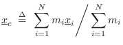
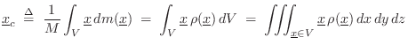
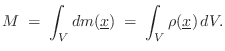
Center of Mass
The center of mass (or centroid) of a rigid body is
found by averaging the spatial points of the body
![]() weighted by the mass
weighted by the mass ![]() of those points:B.12
of those points:B.12
A nice property of the center of mass is that gravity acts on a far-away object as if all its mass were concentrated at its center of mass. For this reason, the center of mass is often called the center of gravity.
Linear Momentum of the Center of Mass
Consider a system of ![]() point-masses
point-masses ![]() , each traveling with
vector velocity
, each traveling with
vector velocity
![]() , and not necessarily rigidly attached to
each other. Then the total momentum of the system is
, and not necessarily rigidly attached to
each other. Then the total momentum of the system is
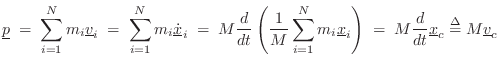
Thus, the momentum
![]() of any collection of masses
of any collection of masses ![]() (including rigid bodies) equals the total mass
(including rigid bodies) equals the total mass ![]() times the
velocity of the center-of-mass.
times the
velocity of the center-of-mass.
Whoops, No Angular Momentum!
The previous result might be surprising since we said at the outset that we were going to decompose the total momentum into a sum of linear plus angular momentum. Instead, we found that the total momentum is simply that of the center of mass, which means any angular momentum that might have been present just went away. (The center of mass is just a point that cannot rotate in a measurable way.) Angular momentum does not contribute to linear momentum, so it provides three new ``degrees of freedom'' (three new energy storage dimensions, in 3D space) that are ``missed'' when considering only linear momentum.
To obtain the desired decomposition of momentum into linear plus angular momentum, we will choose a fixed reference point in space (usually the center of mass) and then, with respect to that reference point, decompose an arbitrary mass-particle travel direction into the sum of two mutually orthogonal vector components: one will be the vector component pointing radially with respect to the fixed point (for the ``linear momentum'' component), and the other will be the vector component pointing tangentially with respect to the fixed point (for the ``angular momentum''), as shown in Fig.B.3. When the reference point is the center of mass, the resultant radial force component gives us the force on the center of mass, which creates linear momentum, while the net tangential component (times distance from the center-of-mass) give us a resultant torque about the reference point, which creates angular momentum. As we saw above, because the tangential force component does not contribute to linear momentum, we can simply sum the external force vectors and get the same result as summing their radial components. These topics will be discussed further below, after some elementary preliminaries.
![\includegraphics[width=1.5in]{eps/rigidbody}](http://www.dsprelated.com/josimages_new/pasp/img2710.png) |
Translational Kinetic Energy
The translational kinetic energy of a collection of masses
![]() is given by
is given by
More generally, the total energy of a collection of masses (including distributed and/or rigidly interconnected point-masses) can be expressed as the sum of the translational and rotational kinetic energies [270, p. 98].
Rotational Kinetic Energy
![\includegraphics[width=1.2in]{eps/masscircle}](http://www.dsprelated.com/josimages_new/pasp/img2715.png) |
The rotational kinetic energy of a rigid assembly of masses (or
mass distribution) is the sum of the rotational kinetic energies of
the component masses. Therefore, consider a point-mass ![]() rotatingB.13 in a circular orbit
of radius
rotatingB.13 in a circular orbit
of radius ![]() and angular velocity
and angular velocity ![]() (radians per second), as
shown in Fig.B.4. To make it a closed system, we can
imagine an effectively infinite mass at the origin
(radians per second), as
shown in Fig.B.4. To make it a closed system, we can
imagine an effectively infinite mass at the origin
![]() . Then the
speed of the mass along the circle is
. Then the
speed of the mass along the circle is ![]() , and its kinetic
energy is
, and its kinetic
energy is
![]() . Since this is what we want
for the rotational kinetic energy of the system, it is
convenient to define it in terms of angular velocity
. Since this is what we want
for the rotational kinetic energy of the system, it is
convenient to define it in terms of angular velocity ![]() in
radians per second. Thus, we write
in
radians per second. Thus, we write
where
is called the mass moment of inertia.
Mass Moment of Inertia
The mass moment of inertia ![]() (or simply moment of
inertia), plays the role of mass in rotational dynamics, as
we saw in
Eq.
(or simply moment of
inertia), plays the role of mass in rotational dynamics, as
we saw in
Eq.![]() (B.7) above.
(B.7) above.
The mass moment of inertia of a rigid body, relative to a given axis of rotation, is given by a weighted sum over its mass, with each mass-point weighted by the square of its distance from the rotation axis. Compare this with the center of mass (§B.4.1) in which each mass-point is weighted by its vector location in space (and divided by the total mass).
Equation (B.8) above gives the moment of inertia for a single point-mass
![]() rotating a distance
rotating a distance ![]() from the axis to be
from the axis to be ![]() . Therefore,
for a rigid collection of point-masses
. Therefore,
for a rigid collection of point-masses ![]() ,
,
![]() ,B.14 the
moment of inertia about a given axis of rotation is obtained by adding
the component moments of inertia:
,B.14 the
moment of inertia about a given axis of rotation is obtained by adding
the component moments of inertia:
where
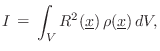
For a continuous mass distribution, the moment of inertia is given by integrating the contribution of each differential mass element:
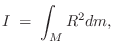 |
(B.10) |
where
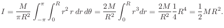
Circular Disk Rotating in Its Own Plane
For example, the moment of inertia for a uniform circular disk of
total mass ![]() and radius
and radius ![]() , rotating in its own plane about a
rotation axis piercing its center, is given by
, rotating in its own plane about a
rotation axis piercing its center, is given by
Circular Disk Rotating About Its Diameter
The moment of inertia for the same circular disk rotating about an axis in the plane of the disk, passing through its center, is given by
![$\displaystyle I = \frac{M}{\pi R^2}\cdot 4\int_0^{\pi/2} \int_0^R [r\cos(\theta)]^2\, r\,dr\,d\theta
= \frac{1}{4}MR^2
$](http://www.dsprelated.com/josimages_new/pasp/img2728.png)
Perpendicular Axis Theorem
In general, for any 2D distribution of mass, the moment of inertia
about an axis orthogonal to the plane of the mass equals the sum of
the moments of inertia about any two mutually orthogonal axes in the
plane of the mass intersecting the first axis. To see this, consider
an arbitrary mass element ![]() having rectilinear coordinates
having rectilinear coordinates
![]() in the plane of the mass. (All three coordinate axes
intersect at a point in the mass-distribution plane.) Then its moment
of inertia about the axis orthogonal to the mass plane is
in the plane of the mass. (All three coordinate axes
intersect at a point in the mass-distribution plane.) Then its moment
of inertia about the axis orthogonal to the mass plane is
![]() while its moment of inertia about coordinate axes
within the mass-plane are respectively
while its moment of inertia about coordinate axes
within the mass-plane are respectively ![]() and
and ![]() .
This, the perpendicular axis theorem is an immediate consequence of
the Pythagorean theorem for right triangles.
.
This, the perpendicular axis theorem is an immediate consequence of
the Pythagorean theorem for right triangles.
Parallel Axis Theorem
Let ![]() denote the moment of inertia for a rotation axis passing
through the center of mass, and let
denote the moment of inertia for a rotation axis passing
through the center of mass, and let ![]() denote
the moment of inertia for a rotation axis parallel to the first
but a distance
denote
the moment of inertia for a rotation axis parallel to the first
but a distance ![]() away from it. Then the parallel axis theorem
says that
away from it. Then the parallel axis theorem
says that
Stretch Rule
Note that the moment of inertia does not change when masses are moved
along a vector parallel to the axis of rotation (see, e.g.,
Eq.![]() (B.9)). Thus, any rigid body may be ``stretched'' or
``squeezed'' parallel to the rotation axis without changing its moment
of inertia. This is known as the stretch rule, and it can be
used to simplify geometry when finding the moment of inertia.
(B.9)). Thus, any rigid body may be ``stretched'' or
``squeezed'' parallel to the rotation axis without changing its moment
of inertia. This is known as the stretch rule, and it can be
used to simplify geometry when finding the moment of inertia.
For example, we saw in §B.4.4 that the moment of inertia
of a point-mass ![]() a distance
a distance ![]() from the axis of rotation is given
by
from the axis of rotation is given
by ![]() . By the stretch rule, the same applies to an ideal
rod of mass
. By the stretch rule, the same applies to an ideal
rod of mass ![]() parallel to and distance
parallel to and distance ![]() from the axis of
rotation.
from the axis of
rotation.
Note that mass can be also be ``stretched'' along the circle of
rotation without changing the moment of inertia for the mass about
that axis. Thus, the point mass ![]() can be stretched out to form a
mass ring at radius
can be stretched out to form a
mass ring at radius ![]() about the axis of rotation without
changing its moment of inertia about that axis. Similarly, the ideal
rod of the previous paragraph can be stretched tangentially to form a
cylinder of radius
about the axis of rotation without
changing its moment of inertia about that axis. Similarly, the ideal
rod of the previous paragraph can be stretched tangentially to form a
cylinder of radius ![]() and mass
and mass ![]() , with its axis of symmetry
coincident with the axis of rotation. In all of these examples, the
moment of inertia is
, with its axis of symmetry
coincident with the axis of rotation. In all of these examples, the
moment of inertia is ![]() about the axis of rotation.
about the axis of rotation.
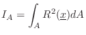
Area Moment of Inertia
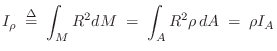
The area moment of inertia is the second moment of an area ![]() around a given axis:
around a given axis:
Comparing with the definition of mass moment of inertia in §B.4.4 above, we see that mass is replaced by area in the area moment of inertia.
In a planar mass distribution with total mass ![]() uniformly
distributed over an area
uniformly
distributed over an area ![]() (i.e., a constant mass density of
(i.e., a constant mass density of
![]() ), the mass moment of inertia
), the mass moment of inertia ![]() is given by the area
moment of inertia
is given by the area
moment of inertia ![]() times mass-density
times mass-density ![]() :
:
Radius of Gyration
For a planar distribution of mass rotating about some axis in the plane of the mass, the radius of gyration is the distance from the axis that all mass can be concentrated to obtain the same mass moment of inertia. Thus, the radius of gyration is the ``equivalent distance'' of the mass from the axis of rotation. In this context, gyration can be defined as rotation of a planar region about some axis lying in the plane.
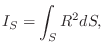
For a bar cross-section with area ![]() , the radius of gyration is given by
, the radius of gyration is given by

where
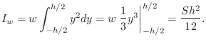
Rectangular Cross-Section
For a rectangular cross-section of height ![]() and width
and width ![]() , area
, area
![]() , the area moment of inertia about the horizontal midline is
given by
, the area moment of inertia about the horizontal midline is
given by
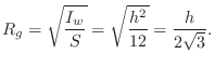
The radius of gyration can be thought of as the ``effective radius'' of the mass distribution with respect to its inertial response to rotation (``gyration'') about the chosen axis.
Most cross-sectional shapes (e.g., rectangular), have at least two radii of gyration. A circular cross-section has only one, and its radius of gyration is equal to half its radius, as shown in the next section.
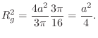
Circular Cross-Section
For a circular cross-section of radius ![]() , Eq.
, Eq.![]() (B.11) tells us
that the squared radius of gyration about any line passing through the
center of the cross-section is given by
(B.11) tells us
that the squared radius of gyration about any line passing through the
center of the cross-section is given by
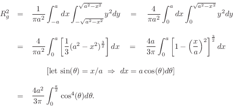
Using the elementrary trig identity
![]() , we readily
derive
, we readily
derive
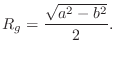
For a circular tube in which the mass of the cross-section lies
within a circular annulus having inner radius ![]() and outer
radius
and outer
radius ![]() , the radius of gyration is given by
, the radius of gyration is given by
Two Masses Connected by a Rod
![\includegraphics[width=1.5in]{eps/massrodmass}](http://www.dsprelated.com/josimages_new/pasp/img2758.png)
As an introduction to the decomposition of rigid-body motion into
translational and rotational components, consider the
simple system shown in Fig.B.5. The excitation force
densityB.15 ![]() can be
applied anywhere between
can be
applied anywhere between ![]() and
and ![]() along the connecting rod.
We will deliver a vertical impulse of momentum to the mass on the
right, and show, among other observations, that the total kinetic
energy is split equally into (1) the rotational kinetic energy
about the center of mass, and (2) the translational kinetic
energy of the total mass, treated as being located at the center of
mass. This is accomplished by defining a new frame of
reference (i.e., a moving coordinate system) that has its origin at
the center of mass.
along the connecting rod.
We will deliver a vertical impulse of momentum to the mass on the
right, and show, among other observations, that the total kinetic
energy is split equally into (1) the rotational kinetic energy
about the center of mass, and (2) the translational kinetic
energy of the total mass, treated as being located at the center of
mass. This is accomplished by defining a new frame of
reference (i.e., a moving coordinate system) that has its origin at
the center of mass.
First, note that the driving-point impedance (§7.1)
``seen'' by the driving force ![]() varies as a function of
varies as a function of ![]() .
At
.
At ![]() , The excitation
, The excitation ![]() sees a ``point mass''
sees a ``point mass'' ![]() , and no
rotation is excited by the force (by symmetry). At
, and no
rotation is excited by the force (by symmetry). At ![]() , on the
other hand, the excitation
, on the
other hand, the excitation
![]() only sees mass
only sees mass ![]() at time
0, because the vertical motion of either point-mass initially only
rotates the other point-mass via the massless connecting rod. Thus,
an observation we can make right away is that the driving point
impedance seen by
at time
0, because the vertical motion of either point-mass initially only
rotates the other point-mass via the massless connecting rod. Thus,
an observation we can make right away is that the driving point
impedance seen by ![]() depends on the striking point
depends on the striking point ![]() and,
away from
and,
away from ![]() , it depends on time
, it depends on time ![]() as well.
as well.
To avoid dealing with a time-varying driving-point impedance, we will
use an impulsive force input at time ![]() . Since momentum is the
time-integral of force (
. Since momentum is the
time-integral of force (
![]() ), our
excitation will be a unit momentum transferred to the two-mass
system at time 0.
), our
excitation will be a unit momentum transferred to the two-mass
system at time 0.
Striking the Rod in the Middle
First, consider
![]() . That is, we apply an
upward unit-force impulse at time 0 in the middle of the rod. The
total momentum delivered in the neighborhood of
. That is, we apply an
upward unit-force impulse at time 0 in the middle of the rod. The
total momentum delivered in the neighborhood of ![]() and
and ![]() is
obtained by integrating the applied force density with respect to time
and position:
is
obtained by integrating the applied force density with respect to time
and position:
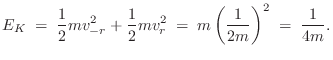
The kinetic energy of the system after time zero is
Striking One of the Masses
Now let
![]() . That is, we apply an impulse
of vertical momentum to the mass on the right at time 0.
. That is, we apply an impulse
of vertical momentum to the mass on the right at time 0.
In this case, the unit of vertical momentum is transferred entirely to the mass on the right, so that
Note that the velocity of the center-of-mass ![]() is the
same as it was when we hit the midpoint of the rod. This is an
important general equivalence: The sum of all external force vectors
acting on a rigid body can be applied as a single resultant force
vector to the total mass concentrated at the center of mass to find
the linear (translational) motion produced. (Recall from §B.4.1
that such a sum is the same as the sum of all radially acting external
force components, since the tangential components contribute only to
rotation and not to translation.)
is the
same as it was when we hit the midpoint of the rod. This is an
important general equivalence: The sum of all external force vectors
acting on a rigid body can be applied as a single resultant force
vector to the total mass concentrated at the center of mass to find
the linear (translational) motion produced. (Recall from §B.4.1
that such a sum is the same as the sum of all radially acting external
force components, since the tangential components contribute only to
rotation and not to translation.)
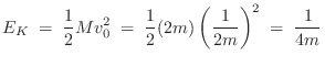
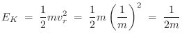
All of the kinetic energy is in the mass on the right just after time zero:
However, after time zero, things get more complicated, because the mass on the left gets dragged into a rotation about the center of mass.
To simplify ongoing analysis, we can define a body-fixed frame
of referenceB.16 having its origin at the center of mass. Let ![]() denote a velocity in this frame. Since the velocity of the center of
mass is
denote a velocity in this frame. Since the velocity of the center of
mass is
![]() , we can convert any velocity
, we can convert any velocity ![]() in the
body-fixed frame to a velocity
in the
body-fixed frame to a velocity ![]() in the original frame by adding
in the original frame by adding
![]() to it, viz.,
to it, viz.,
In the body-fixed frame, all kinetic energy is rotational about
the origin. Recall (Eq.![]() (B.9)) that the moment of inertia for this
system, with respect to the center of mass at
(B.9)) that the moment of inertia for this
system, with respect to the center of mass at ![]() , is
, is
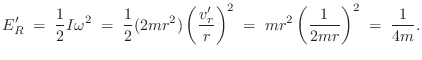
In summary, we defined a moving body-fixed frame having its origin at the center-of-mass, and the total kinetic energy was computed to be
It is important to note that, after time zero, both the linear
momentum of the center-of-mass (
![]() ), and the angular momentum in the body-fixed frame
(
), and the angular momentum in the body-fixed frame
(
![]() ) remain
constant over time.B.17 In the original space-fixed
frame, on the other hand, there is a complex transfer of momentum back
and forth between the masses after time zero.
) remain
constant over time.B.17 In the original space-fixed
frame, on the other hand, there is a complex transfer of momentum back
and forth between the masses after time zero.
Similarly, the translational kinetic energy of the total mass, treated as being concentrated at its center-of-mass, and the rotational kinetic energy in the body-fixed frame, are both constant after time zero, while in the space-fixed frame, kinetic energy transfers back and forth between the two masses. At all times, however, the total kinetic energy is the same in both formulations.
Angular Velocity Vector
When working with rotations, it is convenient to define the
angular-velocity vector as a vector
![]() pointing
along the axis of rotation. There are two directions we could
choose from, so we pick the one corresponding to the right-hand
rule, i.e., when the fingers of the right hand curl in the direction
of the rotation, the thumb points in the direction of the angular
velocity vector.B.18 The
length
pointing
along the axis of rotation. There are two directions we could
choose from, so we pick the one corresponding to the right-hand
rule, i.e., when the fingers of the right hand curl in the direction
of the rotation, the thumb points in the direction of the angular
velocity vector.B.18 The
length
![]() should obviously equal the angular
velocity
should obviously equal the angular
velocity ![]() . It is convenient also to work with a unit-length
variant
. It is convenient also to work with a unit-length
variant
![]() .
.
As introduced in Eq.![]() (B.8) above, the mass moment of inertia is
given by
(B.8) above, the mass moment of inertia is
given by ![]() where
where ![]() is the distance from the (instantaneous)
axis of rotation to the mass
is the distance from the (instantaneous)
axis of rotation to the mass ![]() located at
located at
![]() . In
terms of the angular-velocity vector
. In
terms of the angular-velocity vector
![]() , we can write this as
(see Fig.B.6)
, we can write this as
(see Fig.B.6)
where

![\includegraphics[width=1.5in]{eps/pxov}](http://www.dsprelated.com/josimages_new/pasp/img2806.png) |
Using the vector cross product (defined in the next section),
we will show (in §B.4.17) that ![]() can be written more succinctly as
can be written more succinctly as
Vector Cross Product
The vector cross product (or simply vector product, as
opposed to the scalar product (which is also called the
dot product, or inner product)) is commonly used in
vector calculus--a basic mathematical toolset used in
mechanics [270,258],
acoustics [349], electromagnetism [356], quantum
mechanics, and more. It can be defined symbolically in the form of
a matrix determinant:B.19
![$\displaystyle \left\vert \begin{array}{ccc}
\underline{e}_1 & \underline{e}_2 &...
...ine{e}_3\\ [2pt]
x_1 & x_2 & x_3\\ [2pt]
y_1 & y_2 & y_3
\end{array}\right\vert$](http://www.dsprelated.com/josimages_new/pasp/img2809.png)
![$\displaystyle \left[\begin{array}{ccc}
0 & -x_3 & x_2\\ [2pt]
x_3 & 0 & -x_1\\ ...
...}\right]
\left[\begin{array}{c} x_1 \\ [2pt] x_2 \\ [2pt] x_3\end{array}\right]$](http://www.dsprelated.com/josimages_new/pasp/img2811.png)
where
The second and third lines of Eq.![]() (B.15) make it clear that
(B.15) make it clear that
![]() . This is one example of a host of identities that
one learns in vector calculus and its applications.
. This is one example of a host of identities that
one learns in vector calculus and its applications.
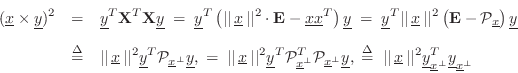
Cross-Product Magnitude
It is a straightforward exercise to show that the cross-product magnitude is equal to the product of the vector lengths times the sine of the angle between them:B.21
where
To derive Eq.![]() (B.16), let's begin with the cross-product in matrix
form as
(B.16), let's begin with the cross-product in matrix
form as
![]() using the first matrix form in the
third line of the cross-product definition in Eq.
using the first matrix form in the
third line of the cross-product definition in Eq.![]() (B.15) above. Then
(B.15) above. Then
where
![]() denotes the identity matrix in
denotes the identity matrix in
![]() ,
,
![]() denotes the orthogonal-projection matrix onto
denotes the orthogonal-projection matrix onto
![]() [451],
[451],
![]() denotes the projection matrix onto
the orthogonal complement of
denotes the projection matrix onto
the orthogonal complement of
![]() ,
,
![]() denotes the component of
denotes the component of
![]() orthogonal to
orthogonal to
![]() , and we used the fact that orthogonal projection matrices
, and we used the fact that orthogonal projection matrices
![]() are idempotent (i.e.,
are idempotent (i.e.,
![]() ) and
symmetric (when real, as we have here) when we replaced
) and
symmetric (when real, as we have here) when we replaced
![]() by
by
![]() above. Finally,
note that the length of
above. Finally,
note that the length of
![]() is
is
![]() , where
, where ![]() is the angle
between the 1D subspaces spanned by
is the angle
between the 1D subspaces spanned by
![]() and
and
![]() in the plane
including both vectors. Thus,
in the plane
including both vectors. Thus,
The direction of the cross-product vector is then taken to be
orthogonal to both
![]() and
and
![]() according to the right-hand
rule. This orthogonality can be checked by verifying that
according to the right-hand
rule. This orthogonality can be checked by verifying that
![]() . The right-hand-rule parity can be checked by
rotating the space so that
. The right-hand-rule parity can be checked by
rotating the space so that
![]() and
and
![]() in
which case
in
which case
![]() . Thus, the cross
product points ``up'' relative to the
. Thus, the cross
product points ``up'' relative to the
![]() plane for
plane for
![]() and ``down'' for
and ``down'' for
![]() .
.
Mass Moment of Inertia as a Cross Product
In Eq.![]() (B.14) above, the mass moment of inertia was expressed
in terms of orthogonal projection as
(B.14) above, the mass moment of inertia was expressed
in terms of orthogonal projection as
![]() , where
, where
![]() . In terms of the vector cross
product, we can now express it as
. In terms of the vector cross
product, we can now express it as
Tangential Velocity as a Cross Product
Referring again to Fig.B.4, we can write the
tangential velocity vector
![]() as a vector cross product of
the angular-velocity vector
as a vector cross product of
the angular-velocity vector
![]() (§B.4.11) and the position
vector
(§B.4.11) and the position
vector
![]() :
:
To see this, let's first check its direction and then its magnitude. By the right-hand rule,
Angular Momentum
The angular momentum of a mass ![]() rotating in a circle of
radius
rotating in a circle of
radius ![]() with angular velocity
with angular velocity ![]() (rad/s), is defined by
(rad/s), is defined by
Relation of Angular to Linear Momentum
Recall (§B.3) that the momentum of a mass ![]() traveling
with velocity
traveling
with velocity ![]() in a straight line is given by
in a straight line is given by
Thus, the angular momentum
Linear momentum can be viewed as a renormalized special case of angular momentum in which the radius of rotation goes to infinity.
Angular Momentum Vector
Like linear momentum, angular momentum is fundamentally a vector in
![]() . The definition of the previous section suffices when the
direction does not change, in which case we can focus only on its
magnitude
. The definition of the previous section suffices when the
direction does not change, in which case we can focus only on its
magnitude ![]() .
.
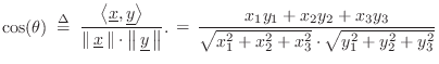
More generally, let
![]() denote the 3-space coordinates
of a point-mass
denote the 3-space coordinates
of a point-mass ![]() , and let
, and let
![]() denote its velocity
in
denote its velocity
in ![]() . Then the instantaneous angular momentum vector
of the mass relative to the origin (not necessarily rotating about a
fixed axis) is given by
. Then the instantaneous angular momentum vector
of the mass relative to the origin (not necessarily rotating about a
fixed axis) is given by
where
For the special case in which
![]() is orthogonal to
is orthogonal to
![]() , as in Fig.B.4, we have that
, as in Fig.B.4, we have that
![]() points, by the right-hand rule, in the direction of the angular
velocity vector
points, by the right-hand rule, in the direction of the angular
velocity vector
![]() (up out of the page), which is
satisfying. Furthermore, its magnitude is given by
(up out of the page), which is
satisfying. Furthermore, its magnitude is given by
In the more general case of an arbitrary mass velocity vector
![]() , we know from §B.4.12 that the magnitude of
, we know from §B.4.12 that the magnitude of
![]() equals the product of the distance from the axis
of rotation to the mass, i.e.,
equals the product of the distance from the axis
of rotation to the mass, i.e.,
![]() , times the length of
the component of
, times the length of
the component of
![]() that is orthogonal to
that is orthogonal to
![]() , i.e.,
, i.e.,
![]() , as needed.
, as needed.
It can be shown that vector angular momentum, as defined, is conserved.B.22 For example, in an orbit, such as that of the moon around the earth, or that of Halley's comet around the sun, the orbiting object speeds up as it comes closer to the object it is orbiting. (See Kepler's laws of planetary motion.) Similarly, a spinning ice-skater spins faster when pulling in arms to reduce the moment of inertia about the spin axis. The conservation of angular momentum can be shown to result from the principle of least action and the isotrophy of space [270, p. 18].
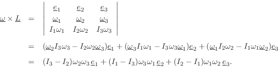
Angular Momentum Vector in Matrix Form
The two cross-products in Eq.![]() (B.19) can be written out with the help
of the vector analysis identityB.23
(B.19) can be written out with the help
of the vector analysis identityB.23
where
![$\displaystyle \mathbf{I}\underline{\omega}\eqsp
\left[\begin{array}{ccc}
I_{1...
...begin{array}{c} \omega_1 \\ [2pt] \omega_2 \\ [2pt] \omega_3\end{array}\right]
$](http://www.dsprelated.com/josimages_new/pasp/img2872.png)
The matrix
The vector angular momentum of a rigid body is obtained by summing the angular momentum of its constituent mass particles. Thus,
In summary, the angular momentum vector
![]() is given by the mass
moment of inertia tensor
is given by the mass
moment of inertia tensor
![]() times the angular-velocity vector
times the angular-velocity vector
![]() representing the axis of rotation.
representing the axis of rotation.
Note that the angular momentum vector
![]() does not in general
point in the same direction as the angular-velocity vector
does not in general
point in the same direction as the angular-velocity vector
![]() . We
saw above that it does in the special case of a point mass traveling
orthogonal to its position vector. In general,
. We
saw above that it does in the special case of a point mass traveling
orthogonal to its position vector. In general,
![]() and
and
![]() point
in the same direction whenever
point
in the same direction whenever
![]() is an eigenvector of
is an eigenvector of
![]() , as will be discussed further below (§B.4.16). In this
case, the rigid body is said to be dynamically balanced.B.24
, as will be discussed further below (§B.4.16). In this
case, the rigid body is said to be dynamically balanced.B.24
Mass Moment of Inertia Tensor
As derived in the previous section, the moment of inertia
tensor, in 3D Cartesian coordinates, is a three-by-three matrix
![]() that can be multiplied by any angular-velocity vector to
produce the corresponding angular momentum vector for either a point
mass or a rigid mass distribution. Note that the origin of the
angular-velocity vector
that can be multiplied by any angular-velocity vector to
produce the corresponding angular momentum vector for either a point
mass or a rigid mass distribution. Note that the origin of the
angular-velocity vector
![]() is always fixed at
is always fixed at
![]() in the space
(typically located at the center of mass). Therefore, the moment of
inertia tensor
in the space
(typically located at the center of mass). Therefore, the moment of
inertia tensor
![]() is defined relative to that origin.
is defined relative to that origin.
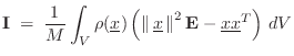
The moment of inertia tensor can similarly be used to compute the
mass moment of inertia for any normalized angular velocity
vector
![]() as
as
Since rotational energy is defined as
We can show Eq.
where again
![]() denotes the three-by-three identity matrix, and
denotes the three-by-three identity matrix, and
which agrees with Eq.
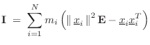
For a collection of ![]() masses
masses ![]() located at
located at
![]() , we
simply sum over their masses to add up the moments of inertia:
, we
simply sum over their masses to add up the moments of inertia:
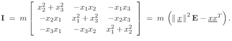
Simple Example
Consider a mass ![]() at
at
![]() . Then the mass moment of inertia
tensor is
. Then the mass moment of inertia
tensor is
![$\displaystyle \mathbf{I}\eqsp m \left(\left\Vert\,\underline{x}\,\right\Vert^2\...
...ay}{ccc}
0 & 0 & 0\\ [2pt]
0 & 1 & 0\\ [2pt]
0 & 0 & 1
\end{array}\right].
$](http://www.dsprelated.com/josimages_new/pasp/img2891.png)
![\begin{displaymath}
I \eqsp \underline{\tilde{\omega}}^T\mathbf{I}\,\underline{\...
...{array}{c} 1 \\ [2pt] 0 \\ [2pt] 0\end{array}\right]m \eqsp 0.
\end{displaymath}](http://www.dsprelated.com/josimages_new/pasp/img2893.png)
![$\displaystyle I \eqsp \underline{\tilde{\omega}}^T\mathbf{I}\,\underline{\tilde...
...]
\left[\begin{array}{c} 0 \\ [2pt] 1 \\ [2pt] 0\end{array}\right] \eqsp m x^2
$](http://www.dsprelated.com/josimages_new/pasp/img2895.png)
Example with Coupled Rotations
Now let the mass ![]() be located at
be located at
![]() so that
so that
![\begin{eqnarray*}
\mathbf{I}&=& m \left(\left\Vert\,\underline{x}\,\right\Vert^2...
... & 0\\ [2pt]
-1 & 1 & 0\\ [2pt]
0 & 0 & 2
\end{array}\right].
\end{eqnarray*}](http://www.dsprelated.com/josimages_new/pasp/img2897.png)
We expect
![]() to yield zero for the moment of inertia, and
sure enough
to yield zero for the moment of inertia, and
sure enough
![]() . Similarly, the vector angular
momentum is zero, since
. Similarly, the vector angular
momentum is zero, since
![]() .
.
For
![]() , the result is
, the result is
![\begin{displaymath}
\mathbf{I}\eqsp
\begin{array}{r}\left[\begin{array}{ccc} 1 ...
...egin{array}{c} 1 \\ [2pt] 0 \\ [2pt] 0\end{array}\right]m = m,
\end{displaymath}](http://www.dsprelated.com/josimages_new/pasp/img2902.png)
Off-Diagonal Terms in Moment of Inertia Tensor
This all makes sense, but what about those ![]() off-diagonal terms in
off-diagonal terms in
![]() ? Consider the vector angular momentum (§B.4.14):
? Consider the vector angular momentum (§B.4.14):
![$\displaystyle \underline{L}\eqsp \mathbf{I}\,\underline{\omega}\eqsp
m\left[\b...
...begin{array}{c} \omega_1 \\ [2pt] \omega_2 \\ [2pt] \omega_3\end{array}\right]
$](http://www.dsprelated.com/josimages_new/pasp/img2907.png)
Principal Axes of Rotation
A principal axis of rotation (or principal direction) is
an eigenvector of the mass moment of inertia tensor (introduced
in the previous section) defined relative to some point (typically the
center of mass). The corresponding eigenvalues are called the
principal moments of inertia.
Because the moment of inertia tensor is defined relative to the point
![]() in the space, the principal axes all pass through that point
(usually the center of mass).
in the space, the principal axes all pass through that point
(usually the center of mass).
As derived above (§B.4.14), the angular momentum vector is given by the moment of inertia tensor times the angular-velocity vector:
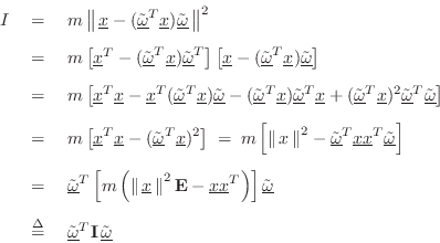
Positive Definiteness of the Moment of Inertia Tensor
From the form of the moment of inertia tensor introduced in Eq.![]() (B.24)
(B.24)
![\begin{eqnarray*}
I &=& \underline{\tilde{\omega}}^T\mathbf{I}\,\underline{\tild...
...\cal P}_{\underline{x}}(\underline{\tilde{\omega}})\right] \ge 0
\end{eqnarray*}](http://www.dsprelated.com/josimages_new/pasp/img2916.png)
since
![]() is unit length, and projecting it onto any other vector
can only shorten it or leave it unchanged. That is,
is unit length, and projecting it onto any other vector
can only shorten it or leave it unchanged. That is,
![]() , with equality occurring for
, with equality occurring for
![]() for any nonzero
for any nonzero
![]() . Zooming out,
of course we expect any moment of inertia
. Zooming out,
of course we expect any moment of inertia ![]() for a positive
mass
for a positive
mass ![]() to be nonnegative. Thus,
to be nonnegative. Thus,
![]() is symmetric
nonnegative definite. If furthermore
is symmetric
nonnegative definite. If furthermore
![]() and
and
![]() are not
collinear, i.e., if there is any nonzero angle between them, then
are not
collinear, i.e., if there is any nonzero angle between them, then
![]() is positive definite (and
is positive definite (and ![]() ). As is well known in
linear algebra [329], real, symmetric, positive-definite
matrices have orthogonal eigenvectors and real, positive
eigenvalues. In this context, the orthogonal eigenvectors are
called the principal axes of rotation. Each corresponding
eigenvalue is the moment of inertia about that principal axis--the
corresponding principal moment of inertia. When angular velocity
vectors
). As is well known in
linear algebra [329], real, symmetric, positive-definite
matrices have orthogonal eigenvectors and real, positive
eigenvalues. In this context, the orthogonal eigenvectors are
called the principal axes of rotation. Each corresponding
eigenvalue is the moment of inertia about that principal axis--the
corresponding principal moment of inertia. When angular velocity
vectors
![]() are expressed as a linear combination of the principal
axes, there are no cross-terms in the moment of inertia tensor--no
so-called products of inertia.
are expressed as a linear combination of the principal
axes, there are no cross-terms in the moment of inertia tensor--no
so-called products of inertia.
The three principal axes are unique when the eigenvalues of
![]() (principal moments of inertia) are distinct. They are
not unique when there are repeated eigenvalues, as in the example
above of a disk rotating about any of its diameters
(§B.4.4). In that example, one principal
axis, the one corresponding to eigenvalue
(principal moments of inertia) are distinct. They are
not unique when there are repeated eigenvalues, as in the example
above of a disk rotating about any of its diameters
(§B.4.4). In that example, one principal
axis, the one corresponding to eigenvalue ![]() , was
, was
![]() (i.e.,
orthogonal to the disk and passing through its center), while any two
orthogonal diameters in the plane of the disk may be chosen as the
other two principal axes (corresponding to the repeated eigenvalue
(i.e.,
orthogonal to the disk and passing through its center), while any two
orthogonal diameters in the plane of the disk may be chosen as the
other two principal axes (corresponding to the repeated eigenvalue
![]() ).
).
Symmetry of the rigid body about any axis
![]() (passing through the
origin) means that
(passing through the
origin) means that
![]() is a principal direction. Such a symmetric
body may be constructed, for example, as a solid of
revolution.B.26In rotational dynamics, this case is known as the symmetric top
[270]. Note that the center of mass will lie
somewhere along an axis of symmetry. The other two principal axes can
be arbitrarily chosen as a mutually orthogonal pair in the (circular)
plane orthogonal to the
is a principal direction. Such a symmetric
body may be constructed, for example, as a solid of
revolution.B.26In rotational dynamics, this case is known as the symmetric top
[270]. Note that the center of mass will lie
somewhere along an axis of symmetry. The other two principal axes can
be arbitrarily chosen as a mutually orthogonal pair in the (circular)
plane orthogonal to the
![]() axis, intersecting at the
axis, intersecting at the
![]() axis. Because of the circular symmetry about
axis. Because of the circular symmetry about
![]() , the two
principal moments of inertia in that plane are equal. Thus the moment
of inertia tensor can be diagonalized to look like
, the two
principal moments of inertia in that plane are equal. Thus the moment
of inertia tensor can be diagonalized to look like
![$\displaystyle \mathbf{I}= \left[\begin{array}{ccc}
I_1 & 0 & 0\\ [2pt]
0 & I_2 & 0\\ [2pt]
0 & 0 & I_2
\end{array}\right],
$](http://www.dsprelated.com/josimages_new/pasp/img2925.png)
Rotational Kinetic Energy Revisited
If a point-mass is located at
![]() and is rotating about an
axis-of-rotation
and is rotating about an
axis-of-rotation
![]() with angular velocity
with angular velocity ![]() , then the
distance from the rotation axis to the mass is
, then the
distance from the rotation axis to the mass is
![]() ,
or, in terms of the vector cross product,
,
or, in terms of the vector cross product,
![]() . The tangential velocity of the mass is
then
. The tangential velocity of the mass is
then ![]() , so that the kinetic energy can be expressed as
(cf. Eq.
, so that the kinetic energy can be expressed as
(cf. Eq.![]() (B.23))
(B.23))
where
In a collection of ![]() masses
masses ![]() having velocities
having velocities
![]() , we of
course sum the individual kinetic energies to get the total kinetic
energy.
, we of
course sum the individual kinetic energies to get the total kinetic
energy.
Finally, we may also write the rotational kinetic energy as half the inner product of the angular-velocity vector and the angular-momentum vector:B.27
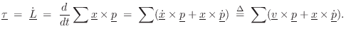
Torque
![\includegraphics[width=1.1in]{eps/torque}](http://www.dsprelated.com/josimages_new/pasp/img2937.png) |
When twisting things, the rotational force we apply about the center
is called a torque (or moment, or moment of
force). Informally, we think of the torque as the tangential
applied force ![]() times the moment arm (length of the
lever arm)
times the moment arm (length of the
lever arm) ![]()
as depicted in Fig.B.7. The moment arm is the distance from the applied force to the point being twisted. For example, in the case of a wrench turning a bolt,
For more general applied forces
![]() , we may compute the
tangential component
, we may compute the
tangential component
![]() by projecting
by projecting
![]() onto the
tangent direction. More precisely, the torque
onto the
tangent direction. More precisely, the torque ![]() about the
origin
about the
origin
![]() applied at a point
applied at a point
![]() may be defined by
may be defined by
where
Note that the torque vector
![]() is orthogonal to both the lever
arm and the tangential-force direction. It thus points in the
direction of the angular velocity vector (along the axis of rotation).
is orthogonal to both the lever
arm and the tangential-force direction. It thus points in the
direction of the angular velocity vector (along the axis of rotation).
The torque magnitude is
Newton's Second Law for Rotations
The rotational version of Newton's law ![]() is
is
where
![\begin{eqnarray*}
\tau &=& \dot{L} \,\eqss \, I\dot{\omega}\,\isdefss \, I\alpha\\ [5pt]
f &=& \dot{p} \,\eqss \, m\dot{v}\,\isdefss \, ma
\end{eqnarray*}](http://www.dsprelated.com/josimages_new/pasp/img2949.png)
To show that Eq.![]() (B.28) results from Newton's second law
(B.28) results from Newton's second law ![]() ,
consider again a mass
,
consider again a mass ![]() rotating at a distance
rotating at a distance ![]() from an axis
of rotation, as in §B.4.3 above, and
let
from an axis
of rotation, as in §B.4.3 above, and
let ![]() denote a tangential force on the mass, and
denote a tangential force on the mass, and ![]() the corresponding tangential acceleration. Then we have, by Newton's
second law,
the corresponding tangential acceleration. Then we have, by Newton's
second law,
In summary, force equals the time-derivative of linear momentum, and torque equals the time-derivative of angular momentum. By Newton's laws, the time-derivative of linear momentum is mass times acceleration, and the time-derivative of angular momentum is the mass moment of inertia times angular acceleration:
Equations of Motion for Rigid Bodies
We are now ready to write down the general equations of motion for
rigid bodies in terms of ![]() for the center of mass and
for the center of mass and
![]() for the rotation of the body about its center of mass.
for the rotation of the body about its center of mass.
As discussed above, it is useful to decompose the motion of a rigid body into
- (1)
- the linear velocity
 of its center of mass, and
- (2)
- its angular velocity
 about its center of mass.
The linear motion is governed by Newton's second law
![]() , where
, where ![]() is the total mass,
is the total mass,
![]() is the
velocity of the center-of-mass, and
is the
velocity of the center-of-mass, and
![]() is the sum of all external
forces on the rigid body. (Equivalently,
is the sum of all external
forces on the rigid body. (Equivalently,
![]() is the sum of the
radial force components pointing toward or away from the center of
mass.) Since this is so straightforward, essentially no harder than
dealing with a point mass, we will not consider it further.
is the sum of the
radial force components pointing toward or away from the center of
mass.) Since this is so straightforward, essentially no harder than
dealing with a point mass, we will not consider it further.
The angular motion is governed the rotational version of Newton's second law introduced in §B.4.19:
where
The driving torque
![]() is given by the resultant moment of
the external forces, using Eq.
is given by the resultant moment of
the external forces, using Eq.![]() (B.27) for each external force to
obtain its contribution to the total moment. In other words, the
external moments (tangential forces times moment arms) sum up for the
net torque just like the radial force components summed to produce the
net driving force on the center of mass.
(B.27) for each external force to
obtain its contribution to the total moment. In other words, the
external moments (tangential forces times moment arms) sum up for the
net torque just like the radial force components summed to produce the
net driving force on the center of mass.
Body-Fixed and Space-Fixed Frames of Reference
Rotation is always about some (instantaneous) axis of rotation that is
free to change over time. It is convenient to express rotations in a
coordinate system having its origin (
![]() ) located at the
center-of-mass of the rigid body (§B.4.1), and its coordinate axes
aligned along the principal directions for the body (§B.4.16).
This body-fixed frame then moves within a stationary
space-fixed frame (or ``star frame'').
) located at the
center-of-mass of the rigid body (§B.4.1), and its coordinate axes
aligned along the principal directions for the body (§B.4.16).
This body-fixed frame then moves within a stationary
space-fixed frame (or ``star frame'').
In Eq.![]() (B.29) above, we wrote down Newton's second law for angular
motion in the body-fixed frame, i.e., the coordinate system
having its origin at the center of mass. Furthermore, it is simplest
(
(B.29) above, we wrote down Newton's second law for angular
motion in the body-fixed frame, i.e., the coordinate system
having its origin at the center of mass. Furthermore, it is simplest
(
![]() is diagonal) when its axes lie along principal directions
(§B.4.16).
is diagonal) when its axes lie along principal directions
(§B.4.16).
As an example of a local body-fixed coordinate system, consider a spinning top. In the body-fixed frame, the ``vertical'' axis coincides with the top's axis of rotation (spin). As the top loses rotational kinetic energy due to friction, the top's rotation-axis precesses around a circle, as observed in the space-fixed frame. The other two body-fixed axes can be chosen as any two mutually orthogonal axes intersecting each other (and the spin axis) at the center of mass, and lying in the plane orthogonal to the spin axis. The space-fixed frame is of course that of the outside observer's inertial frameB.28in which the top is spinning.
Angular Motion in the Space-Fixed Frame
Let's now consider angular motion in the presence of linear motion of the center of mass. In general, we have [270]
Euler's Equations for Rotations in the Body-Fixed Frame
Suppose now that the body-fixed frame is rotating in the space-fixed
frame with angular velocity
![]() . Then the total torque on the rigid
body becomes [270]
. Then the total torque on the rigid
body becomes [270]
Similarly, the total external forces on the center of mass become
![$\displaystyle \underline{L}\eqsp \left[\begin{array}{c} I_1\omega_1 \\ [2pt] I_2\omega_2 \\ [2pt] I_3\omega_3\end{array}\right]
$](http://www.dsprelated.com/josimages_new/pasp/img2969.png)
Substituting this result into Eq.![]() (B.30), we obtain the following
equations of angular motion for an object rotating in the body-fixed
frame defined by its three principal axes of rotation:
(B.30), we obtain the following
equations of angular motion for an object rotating in the body-fixed
frame defined by its three principal axes of rotation:
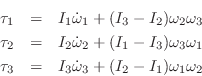
These are call Euler's
equations:B.29Since these equations are in the body-fixed frame, ![]() is the mass
moment of inertia about principal axis
is the mass
moment of inertia about principal axis ![]() , and
, and ![]() is the
angular velocity about principal axis
is the
angular velocity about principal axis ![]() .
.
Examples
For a uniform sphere, the cross-terms disappear and the moments of
inertia are all the same, leaving
![]() , for
, for ![]() .
Since any three orthogonal vectors can serve as eigenvectors of the
moment of inertia tensor, we have that, for a uniform sphere, any
three orthogonal axes can be chosen as principal axes.
.
Since any three orthogonal vectors can serve as eigenvectors of the
moment of inertia tensor, we have that, for a uniform sphere, any
three orthogonal axes can be chosen as principal axes.
For a cylinder that is not spinning about its axis, we similarly
obtain two uncoupled equations
![]() , for
, for ![]() , given
, given
![]() (no spin). Note, however, that if we replace the
circular cross-section of the cylinder by an ellipse, then
(no spin). Note, however, that if we replace the
circular cross-section of the cylinder by an ellipse, then
![]() and there is a coupling term that drives
and there is a coupling term that drives
![]() (unless
(unless ![]() happens to cancel it).
happens to cancel it).
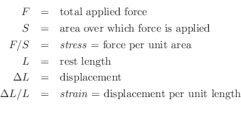
Properties of Elastic Solids
Young's Modulus
Young's modulus can be thought of as the spring constant
for solids. Consider an ideal rod (or bar) of length ![]() and
cross-sectional area
and
cross-sectional area ![]() . Suppose we apply a force
. Suppose we apply a force ![]() to the face of
area
to the face of
area ![]() , causing a displacement
, causing a displacement ![]() along the axis of the rod.
Then Young's modulus
along the axis of the rod.
Then Young's modulus ![]() is given by
is given by

For wood, Young's modulus ![]() is on the order of
is on the order of ![]() N/m
N/m![]() .
For aluminum, it is around
.
For aluminum, it is around ![]() (a bit higher than glass which is near
(a bit higher than glass which is near
![]() ), and structural steel has
), and structural steel has
![]() [180].
[180].
Young's Modulus as a Spring Constant
Recall (§B.1.3) that Hooke's Law defines a spring
constant ![]() as the applied force
as the applied force ![]() divided by the spring
displacement
divided by the spring
displacement ![]() , or
, or ![]() . An elastic solid can be viewed as a
bundle of ideal springs. Consider, for example, an ideal
bar (a rectangular solid in which one dimension, usually its
longest, is designated its length
. An elastic solid can be viewed as a
bundle of ideal springs. Consider, for example, an ideal
bar (a rectangular solid in which one dimension, usually its
longest, is designated its length ![]() ), and consider compression by
), and consider compression by
![]() along the length dimension. The length of each spring in
the bundle is the length of the bar, so that each spring constant
along the length dimension. The length of each spring in
the bundle is the length of the bar, so that each spring constant ![]() must be inversely proportional to
must be inversely proportional to ![]() ; in particular, each doubling of
length
; in particular, each doubling of
length ![]() doubles the length of each ``spring'' in the bundle, and
therefore halves its stiffness. As a result, it is useful to
normalize displacement
doubles the length of each ``spring'' in the bundle, and
therefore halves its stiffness. As a result, it is useful to
normalize displacement ![]() by length
by length ![]() and use relative
displacement
and use relative
displacement
![]() . We need displacement per unit length
because we have a constant spring compliance per unit length.
. We need displacement per unit length
because we have a constant spring compliance per unit length.
The number of springs in parallel is proportional to the
cross-sectional area ![]() of the bar. Therefore, the force applied to
each spring is proportional to the total applied force
of the bar. Therefore, the force applied to
each spring is proportional to the total applied force ![]() divided by
the cross-sectional area
divided by
the cross-sectional area ![]() . Thus, Hooke's law for each spring in the
bundle can be written
. Thus, Hooke's law for each spring in the
bundle can be written

We may say that Young's modulus is the Hooke's-law spring constant for the spring made from a specifically cut section of the solid material, cut to length 1 and cross-sectional area 1. The shape of the cross-sectional area does not matter since all displacement is assumed to be longitudinal in this model.
String Tension
The tension of a vibrating string is the force ![]() used
to stretch it. It is therefore directed along the axis of the string.
A force
used
to stretch it. It is therefore directed along the axis of the string.
A force ![]() must be applied at the endpoint on the right, and a force
must be applied at the endpoint on the right, and a force
![]() is applied at the endpoint on the left. Each point interior to
the string is pulled equally to the left and right,
i.e., the net force on an interior point is
is applied at the endpoint on the left. Each point interior to
the string is pulled equally to the left and right,
i.e., the net force on an interior point is
![]() . (A nonzero
force on a massless point would produce an infinite acceleration.)
. (A nonzero
force on a massless point would produce an infinite acceleration.)
If the cross-sectional area of the string is ![]() , then the tension is
given by the stress on the string times
, then the tension is
given by the stress on the string times ![]() .
.
Wave Equation for the Vibrating String
Consider an elastic string under tension which is at rest along the
![]() dimension. Let
dimension. Let
![]() ,
,
![]() , and
, and
![]() denote the unit vectors in
the
denote the unit vectors in
the ![]() ,
, ![]() , and
, and ![]() directions, respectively. When a wave is
present, a point
directions, respectively. When a wave is
present, a point
![]() originally at
originally at ![]() along the string is
displaced to some point
along the string is
displaced to some point
![]() specified by the displacement
vector
specified by the displacement
vector
The displacement of a neighboring point originally at
![]() along the string can be specified as
along the string can be specified as
Let ![]() denote string tension along
denote string tension along ![]() when the string is at rest, and
when the string is at rest, and
![]() denote the vector tension at the point
denote the vector tension at the point
![]() in the present displaced
scenario under analysis. The net vector force acting on the infinitesimal
string element between points
in the present displaced
scenario under analysis. The net vector force acting on the infinitesimal
string element between points
![]() and
and
![]() is given by the vector sum of
the force
is given by the vector sum of
the force
![]() at
at
![]() and the force
and the force
![]() at
at
![]() , that is,
, that is,
![]() . If the string
has stiffness, the two forces will in general not be tangent to the string
at these points. The mass of the infinitesimal string element is
. If the string
has stiffness, the two forces will in general not be tangent to the string
at these points. The mass of the infinitesimal string element is
![]() ,
where
,
where ![]() denotes the mass per unit length of the string at rest. Applying
Newton's second law gives
denotes the mass per unit length of the string at rest. Applying
Newton's second law gives

where
The next step is to express the force
![]() in terms of the tension
in terms of the tension
![]() of the string at rest, the elastic constant of the string, and
geometrical factors. The displaced string element
of the string at rest, the elastic constant of the string, and
geometrical factors. The displaced string element
![]() is the
vector
is the
vector
![$\displaystyle \left[\mathbf{i}\left(1+\frac{\partial \xi}{\partial x}\right)+
\...
...artial \eta}{\partial x} +
\mathbf{k}\frac{\partial \zeta}{\partial x}\right]dx$](http://www.dsprelated.com/josimages_new/pasp/img3011.png)
having magnitude
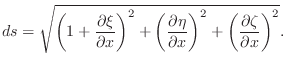
Non-Stiff String
Let's now assume the string is perfectly flexible (zero stiffness) so
that the direction of the force vector
![]() is given by the unit
vector
is given by the unit
vector
![]() tangent to the string. (To accommodate
stiffness, it would be necessary to include a force component at right
angles to the string which depends on the curvature and stiffness of
the string.) The magnitude of
tangent to the string. (To accommodate
stiffness, it would be necessary to include a force component at right
angles to the string which depends on the curvature and stiffness of
the string.) The magnitude of
![]() at any position is the rest
tension
at any position is the rest
tension ![]() plus the incremental tension needed to stretch it the
fractional amount
plus the incremental tension needed to stretch it the
fractional amount
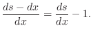
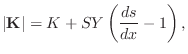
![$\displaystyle \mathbf{K}= \left[K+ SY\left(\frac{ds}{dx} - 1\right)\right]\frac{d{\bf s}}{ds}$](http://www.dsprelated.com/josimages_new/pasp/img3016.png)
where no geometrical limitations have yet been placed on the magnitude of
The four equations (B.31) through (B.35) can be combined into a single vector wave equation that expresses the propagation of waves on the string having three displacement components. This differential equation is nonlinear, so that superposition no longer holds. Furthermore, the three displacement components of the wave are coupled together at all points along the string, so that the wave equation is no longer separable into three independent 1D wave equations.
To obtain a linear, separable wave equation, it is necessary to assume
that the strains
![]() ,
,
![]() , and
, and
![]() be
small compared with unity. This is the same assumption
(
be
small compared with unity. This is the same assumption
(
![]() ) necessary to derive the
usual wave equation for transverse vibrations only in the
) necessary to derive the
usual wave equation for transverse vibrations only in the ![]() -
-![]() plane.
plane.
When (B.35) is expanded into a Taylor series in the strains, and when only the first-order terms are retained, we obtain
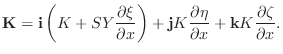 |
(B.36) |
This is the linearized wave equation for the string, based only on the assumptions of elasticity of the string, and strain magnitudes much less than unity. Using this linearized equation for the force
 |
(B.37) | ||
 |
(B.38) | ||
 |
(B.39) |
where
In summary, the two transverse wave components and the longitudinal component may be considered independent (i.e., ``superposition'' holds with respect to vibrations in these three dimensions of vibration) provided powers higher than 1 of the strains (relative displacement) can be neglected, i.e.,
 and
and
Wave Momentum
The physical forward momentum carried by a transverse wave along a string is conveyed by a secondary longitudinal wave [391].
A less simplified wave equation which
supports longitudinal wave momentum is given by [391, Eqns. 38ab]
| (B.40) | |||
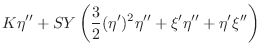 |
(B.41) | ||
| (B.42) |
where
| (B.43) | |||
| (B.44) |
(See also Eq.
Physically, the rising edge of a transverse wave generates a longitudinal displacement in the direction of wave travel that propagates ahead at a much higher speed (typically an order of magnitude faster). The falling edge of the transverse wave then cancels this forward displacement as it passes by. See [391] for further details (including computer simulations).
Properties of Gases
Particle Velocity of a Gas
The particle velocity of a gas flow at any point can be defined as the average velocity (in meters per second, m/s) of the air molecules passing through a plane cutting orthogonal to the flow. The term ``velocity'' in this book, when referring to air, means ``particle velocity.''
It is common in acoustics to denote particle velocity by lower-case
![]() .
.
Volume Velocity of a Gas
The volume velocity ![]() of a gas flow is defined as particle
velocity
of a gas flow is defined as particle
velocity ![]() times the cross-sectional area
times the cross-sectional area ![]() of the flow, or
of the flow, or
When a flow is confined within an enclosed channel, as it is in an
acoustic tube, volume velocity is conserved when the tube
changes cross-sectional area, assuming the density ![]() remains
constant. This follows directly from conservation of mass in a flow:
The total mass passing a given point
remains
constant. This follows directly from conservation of mass in a flow:
The total mass passing a given point ![]() along the flow is given by
the mass density
along the flow is given by
the mass density ![]() times the integral of the volume volume
velocity at that point, or
times the integral of the volume volume
velocity at that point, or
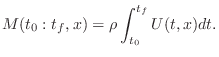
As a simple example, consider a constant flow through two cylindrical
acoustic tube sections having cross-sectional areas ![]() and
and ![]() ,
respectively. If the particle velocity in cylinder 1 is
,
respectively. If the particle velocity in cylinder 1 is ![]() , then
the particle velocity in cylinder 2 may be found by solving
, then
the particle velocity in cylinder 2 may be found by solving
It is common in the field of acoustics to denote volume velocity by an
upper-case ![]() . Thus, for the two-cylinder acoustic tube example above,
we would define
. Thus, for the two-cylinder acoustic tube example above,
we would define
![]() and
and
![]() , so that
, so that
Pressure is Confined Kinetic Energy
According the kinetic theory of ideal gases [180], air pressure can be defined as the average momentum transfer per unit area per unit time due to molecular collisions between a confined gas and its boundary. Using Newton's second law, this pressure can be shown to be given by one third of the average kinetic energy of molecules in the gas.
Proof: This is a classical result from the kinetic theory of gases
[180]. Let ![]() be the total mass of a gas
confined to a rectangular volume
be the total mass of a gas
confined to a rectangular volume ![]() , where
, where ![]() is the area of
one side and
is the area of
one side and ![]() the distance to the opposite side. Let
the distance to the opposite side. Let
![]() denote the average molecule velocity in the
denote the average molecule velocity in the ![]() direction. Then the
total net molecular momentum in the
direction. Then the
total net molecular momentum in the ![]() direction is given by
direction is given by
![]() . Suppose the momentum
. Suppose the momentum
![]() is directed
against a face of area
is directed
against a face of area ![]() . A rigid-wall elastic collision by a mass
. A rigid-wall elastic collision by a mass
![]() traveling into the wall at velocity
traveling into the wall at velocity
![]() imparts a momentum of
magnitude
imparts a momentum of
magnitude
![]() to the wall (because the momentum of the mass is
changed from
to the wall (because the momentum of the mass is
changed from
![]() to
to
![]() , and momentum is conserved).
The average momentum-transfer per unit area is therefore
, and momentum is conserved).
The average momentum-transfer per unit area is therefore
![]() at any instant in time. To obtain the definition of pressure, we need
only multiply by the average collision rate, which is given by
at any instant in time. To obtain the definition of pressure, we need
only multiply by the average collision rate, which is given by
![]() . That is, the average
. That is, the average ![]() -velocity divided by the
round-trip distance along the
-velocity divided by the
round-trip distance along the ![]() dimension gives the collision rate
at either wall bounding the
dimension gives the collision rate
at either wall bounding the ![]() dimension. Thus, we obtain
dimension. Thus, we obtain
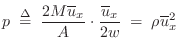
Bernoulli Equation
In an ideal inviscid, incompressible flow, we have, by conservation of energy,
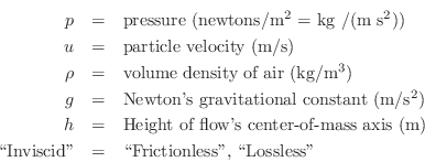
This basic energy conservation law was published in 1738 by Daniel Bernoulli in his classic work Hydrodynamica.
From §B.7.3, we have that the pressure of a gas is
proportional to the average kinetic energy of the molecules making up
the gas. Therefore, when a gas flows at a constant height ![]() , some
of its ``pressure kinetic energy'' must be given to the kinetic energy
of the flow as a whole. If the mean height of the flow changes, then
kinetic energy trades with potential energy as well.
, some
of its ``pressure kinetic energy'' must be given to the kinetic energy
of the flow as a whole. If the mean height of the flow changes, then
kinetic energy trades with potential energy as well.
Bernoulli Effect
The Bernoulli effect provides that, when a gas such as air flows, its pressure drops. This is the basis for how aircraft wings work: The cross-sectional shape of the wing, called an aerofoil (or airfoil), forces air to follow a longer path over the top of the wing, thereby speeding it up and creating a net upward force called lift.
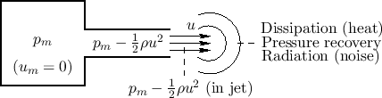
Figure B.8 illustrates the Bernoulli effect for the case
of a reservoir at constant pressure ![]() (``mouth pressure'') driving
an acoustic tube. Any flow inside the ``mouth'' is neglected. Within the
acoustic channel, there is a flow with constant particle velocity
(``mouth pressure'') driving
an acoustic tube. Any flow inside the ``mouth'' is neglected. Within the
acoustic channel, there is a flow with constant particle velocity ![]() .
To conserve energy, the pressure within the acoustic channel must drop
down to
.
To conserve energy, the pressure within the acoustic channel must drop
down to
![]() . That is, the flow kinetic energy subtracts
from the pressure kinetic energy within the channel.
. That is, the flow kinetic energy subtracts
from the pressure kinetic energy within the channel.
For a more detailed derivation of the Bernoulli effect, see, e.g., [179]. Further discussion of its relevance in musical acoustics is given in [144,197].
Air Jets
Referring again to Fig.B.8, the gas flow exiting the acoustic tube is shown as forming a jet. The jet ``carries its own pressure'' until it dissipates in some form, such as any combination of the following:
- heat (now allowing for ``friction'' in the flow),
- vortices (angular momentum),
- radiation (sound waves), or
- pressure recovery.
For a summary of more advanced aeroacoustics, including consideration of vortices, see [196]. In addition, basic textbooks on fluid mechanics are relevant [171].
Acoustic Intensity
Acoustic intensity may be defined by
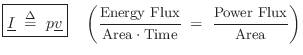
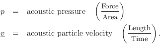
For a plane traveling wave, we have

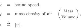
Therefore, in a plane wave,
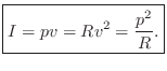
Acoustic Energy Density
The two forms of energy in a wave are kinetic and
potential. Denoting them at a particular time ![]() and position
and position
![]() by
by
![]() and
and
![]() , respectively, we can write them in
terms of velocity
, respectively, we can write them in
terms of velocity ![]() and wave impedance
and wave impedance ![]() as follows:
as follows:
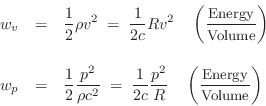
More specifically, ![]() and
and ![]() may be called the acoustic kinetic
energy density and the acoustic potential energy density, respectively.
may be called the acoustic kinetic
energy density and the acoustic potential energy density, respectively.
At each point in a plane wave, we have
![]() (pressure equals wave-impedance times velocity), and so
(pressure equals wave-impedance times velocity), and so
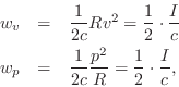
where
![]() denotes the acoustic
intensity (pressure times velocity) at time
denotes the acoustic
intensity (pressure times velocity) at time ![]() and position
and position
![]() .
Thus, half of the acoustic intensity
.
Thus, half of the acoustic intensity ![]() in a plane wave is kinetic,
and the other half is potential:B.30
in a plane wave is kinetic,
and the other half is potential:B.30
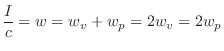
Energy Decay through Lossy Boundaries
Since the acoustic energy density ![]() is the energy per unit
volume in a 3D sound field, it follows that the total energy of the
field is given by integrating over the volume:
is the energy per unit
volume in a 3D sound field, it follows that the total energy of the
field is given by integrating over the volume:
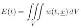
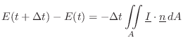
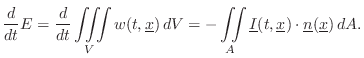
Sabine's theory of acoustic energy decay in reverberant room impulse responses can be derived using this conservation relation as a starting point.
Ideal Gas Law
The ideal gas law can be written as
where
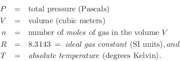
The alternate form ![]() comes from the statistical
mechanics derivation in which
comes from the statistical
mechanics derivation in which ![]() is the number of gas molecules in
the volume, and
is the number of gas molecules in
the volume, and ![]() is Boltzmann's constant. In this
formulation (the kinetic theory of ideal gases), the
average kinetic
energy of the gas molecules is given by
is Boltzmann's constant. In this
formulation (the kinetic theory of ideal gases), the
average kinetic
energy of the gas molecules is given by ![]() . Thus,
temperature is proportional to average kinetic energy of the
gas molecules, where the kinetic energy of a molecule
. Thus,
temperature is proportional to average kinetic energy of the
gas molecules, where the kinetic energy of a molecule ![]() with
translational speed
with
translational speed ![]() is given by
is given by ![]() .
.
In an ideal gas, the molecules are like little rubber balls (or rubbery assemblies of rubber balls) in a weightless vacuum, colliding with each other and the walls elastically and losslessly (an ``ideal rubber''). Electromagnetic forces among the molecules are neglected, other than the electron-orbital repulsion producing the elastic collisions; in other words, the molecules are treated as electrically neutral far away. (Gases of ionized molecules are called plasmas.)
The mass ![]() of the gas in volume
of the gas in volume ![]() is given by
is given by ![]() , where
, where ![]() is
the molar mass of the gass (about 29 g per mole for air). The
air density is thus
is
the molar mass of the gass (about 29 g per mole for air). The
air density is thus ![]() so that we can write
so that we can write

We normally do not need to consider the (nonlinear) ideal gas law in
audio acoustics because it is usually linearized about some
ambient pressure ![]() . The physical pressure is then
. The physical pressure is then ![]() , where
, where
![]() is the usual acoustic pressure-wave variable. That is, we are
only concerned with small pressure perturbations
is the usual acoustic pressure-wave variable. That is, we are
only concerned with small pressure perturbations ![]() in typical
audio acoustics situations, so that, for example, variations in volume
in typical
audio acoustics situations, so that, for example, variations in volume
![]() and density
and density ![]() can be neglected. Notable exceptions include
brass instruments which can achieve nonlinear sound-pressure regions,
especially near the mouthpiece [198,52].
Additionally, the aeroacoustics of air jets is nonlinear
[196,530,531,532,102,101].
can be neglected. Notable exceptions include
brass instruments which can achieve nonlinear sound-pressure regions,
especially near the mouthpiece [198,52].
Additionally, the aeroacoustics of air jets is nonlinear
[196,530,531,532,102,101].
Isothermal versus Isentropic
If air compression/expansion were isothermal (constant
temperature ![]() ), then, according to the ideal gas law
), then, according to the ideal gas law ![]() , the
pressure
, the
pressure ![]() would simply be proportional to density
would simply be proportional to density ![]() . It turns
out, however, that heat diffusion is much slower than audio acoustic
vibrations. As a result, air compression/expansion is much closer to
isentropic (constant entropy
. It turns
out, however, that heat diffusion is much slower than audio acoustic
vibrations. As a result, air compression/expansion is much closer to
isentropic (constant entropy ![]() ) in normal acoustic
situations. (An isentropic process is also called a reversible
adiabatic process.) This means that when air is compressed by
shrinking its volume
) in normal acoustic
situations. (An isentropic process is also called a reversible
adiabatic process.) This means that when air is compressed by
shrinking its volume ![]() , for example, not only does the pressure
, for example, not only does the pressure ![]() increase (§B.7.3), but the temperature
increase (§B.7.3), but the temperature ![]() increases as
well (as quantified in the next section). In a constant-entropy
compression/expansion, temperature changes are not given time to
diffuse away to thermal equilibrium. Instead, they remain largely
frozen in place. Compressing air heats it up, and relaxing the
compression cools it back down.
increases as
well (as quantified in the next section). In a constant-entropy
compression/expansion, temperature changes are not given time to
diffuse away to thermal equilibrium. Instead, they remain largely
frozen in place. Compressing air heats it up, and relaxing the
compression cools it back down.
Adiabatic Gas Constant
The relative amount of compression/expansion energy that goes into
temperature ![]() versus pressure
versus pressure ![]() can be characterized by the heat capacity ratio
can be characterized by the heat capacity ratio

In terms of ![]() , we have
, we have
where
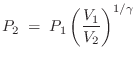
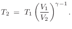
The value
![]() is typical for any diatomic
gas.B.31 Monatomic inert gases, on the other hand,
such as Helium, Neon, and Argon, have
is typical for any diatomic
gas.B.31 Monatomic inert gases, on the other hand,
such as Helium, Neon, and Argon, have
![]() . Carbon
dioxide, which is triatomic, has a heat capacity ratio
. Carbon
dioxide, which is triatomic, has a heat capacity ratio
![]() . We see that more complex molecules have lower
. We see that more complex molecules have lower ![]() values because they can store heat in more degrees of freedom.
values because they can store heat in more degrees of freedom.
Heat Capacity of Ideal Gases
In statistical thermodynamics [175,138],
it is derived that each molecular degree of freedom contributes ![]() to the molar heat capacity of an ideal gas, where again
to the molar heat capacity of an ideal gas, where again ![]() is the
ideal gas constant.
is the
ideal gas constant.
An ideal monatomic gas molecule (negligible spin) has only
three degrees of freedom: its kinetic energy in the three spatial
dimensions. Therefore,
![]() . This means we expect
. This means we expect
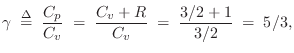
For an ideal diatomic gas molecule such as air, which can be pictured as a ``bar bell'' configuration of two rubber balls, two additional degrees of freedom are added, both associated with spinning the molecule about an axis orthogonal to the line connecting the atoms, and piercing its center of mass. There are two such axes. Spinning about the connecting axis is neglected because the moment of inertia is so much smaller in that case. Thus, for diatomic gases such as dry air, we expect
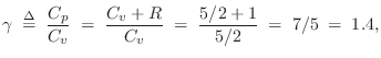
Speed of Sound in Air
The speed of sound in a gas depends primarily on the temperature, and can be estimated using the following formula from the kinetic theory of gases:B.33
Air Absorption
This section provides some further details regarding acoustic air
absorption [318]. For a plane wave, the decline of
acoustic intensity as a function of propagation distance ![]() is given
by
is given
by
Tables B.1 and B.2 (adapted from [314]) give some typical values for air.
| ||||||||||||||||||||||||||||||
| ||||||||||||||||||||||||||||||
There is also a (weaker) dependence of air absorption on temperature [183].
Theoretical models of energy loss in a gas are developed in Morse and
Ingard [318, pp. 270-285]. Energy loss is caused by
viscosity, thermal diffusion, rotational
relaxation, vibration relaxation, and boundary losses
(losses due to heat conduction and viscosity at a wall or other
acoustic boundary). Boundary losses normally dominate by several
orders of magnitude, but in resonant modes, which have nodes along the
boundaries, interior losses dominate, especially for polyatomic gases
such as air.B.34 For air having moderate amounts of water
vapor (![]() ) and/or carbon dioxide (
) and/or carbon dioxide (![]() ), the loss and dispersion
due to
), the loss and dispersion
due to ![]() and
and ![]() vibration relaxation hysteresis becomes the
largest factor [318, p. 300]. The vibration here
is that of the molecule itself, accumulated over the course of many
collisions with other molecules. In this context, a diatomic molecule
may be modeled as two masses connected by an ideal spring. Energy
stored in molecular vibration typically dominates over that stored in
molecular rotation, for polyatomic gas molecules [318, p.
300]. Thus, vibration relaxation hysteresis is a loss
mechanism that converts wave energy into heat.
vibration relaxation hysteresis becomes the
largest factor [318, p. 300]. The vibration here
is that of the molecule itself, accumulated over the course of many
collisions with other molecules. In this context, a diatomic molecule
may be modeled as two masses connected by an ideal spring. Energy
stored in molecular vibration typically dominates over that stored in
molecular rotation, for polyatomic gas molecules [318, p.
300]. Thus, vibration relaxation hysteresis is a loss
mechanism that converts wave energy into heat.
In a resonant mode, the attenuation per wavelength due to vibration
relaxation is greatest when the sinusoidal period (of the resonance)
is equal to ![]() times the time-constant for vibration-relaxation.
The relaxation time-constant for oxygen is on the order of one
millisecond. The presence of water vapor (or other impurities)
decreases the vibration relaxation time, yielding loss maxima at
frequencies above 1000 rad/sec. The energy loss approaches zero as
the frequency goes to infinity (wavelength to zero).
times the time-constant for vibration-relaxation.
The relaxation time-constant for oxygen is on the order of one
millisecond. The presence of water vapor (or other impurities)
decreases the vibration relaxation time, yielding loss maxima at
frequencies above 1000 rad/sec. The energy loss approaches zero as
the frequency goes to infinity (wavelength to zero).
Under these conditions, the speed of sound is approximately that of dry air below the maximum-loss frequency, and somewhat higher above. Thus, the humidity level changes the dispersion cross-over frequency of the air in a resonant mode.
Wave Equation in Higher Dimensions
The wave equation in 1D, 2D, or 3D may be written as

where, in 3D,

Plane Waves in Air
Figure B.9 shows a 2D ![]() cross-section of a snapshot (in time)
of the sinusoidal plane wave
cross-section of a snapshot (in time)
of the sinusoidal plane wave
![\includegraphics[width=\twidth]{eps/planewave}](http://www.dsprelated.com/josimages_new/pasp/img3149.png) |
Figure B.10 depicts a more mathematical schematic of a sinusoidal plane wave traveling toward the upper-right of the figure. The dotted lines indicate the crests (peak amplitude location) along the wave.
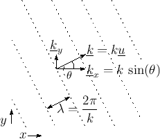
The direction of travel and spatial frequency are indicated by the
vector wavenumber
![]() , as discussed in in the following section.
, as discussed in in the following section.
Vector Wavenumber
Mathematically, a sinusoidal plane wave, as in Fig.B.9 or Fig.B.10, can be written as
where p(t,x) is the pressure at time
![$\displaystyle \underline{k}\eqsp \left[\begin{array}{c} k_x \\ [2pt] k_y \\ [2p...
... \cos{\beta} \\ [2pt] \cos{\gamma}\end{array}\right] \isdefs k\,\underline{u},
$](http://www.dsprelated.com/josimages_new/pasp/img3153.png)
-
 (unit) vector of direction cosines
-
 (scalar) wavenumber along travel
direction
(scalar) wavenumber along travel
direction
- wavenumber along the travel direction in its magnitude

- travel direction in its orientation

To see that the vector wavenumber
![]() has the claimed
properties, consider that the orthogonal projection of any
vector
has the claimed
properties, consider that the orthogonal projection of any
vector
![]() onto a vector collinear with
onto a vector collinear with
![]() is given by
is given by
![]() [451].B.35Thus,
[451].B.35Thus,
![]() is the component of
is the component of
![]() lying along the
direction of wave propagation indicated by
lying along the
direction of wave propagation indicated by
![]() . The norm of this
component is
. The norm of this
component is
![]() , since
, since
![]() is
unit-norm by construction. More generally,
is
unit-norm by construction. More generally,
![]() is the
signed length (in meters) of the component of
is the
signed length (in meters) of the component of
![]() along
along
![]() .
This length times wavenumber
.
This length times wavenumber ![]() gives the spatial phase advance along
the wave, or,
gives the spatial phase advance along
the wave, or,
![]() .
.
For another point of view, consider the plane wave
![]() ,
which is the varying portion of the general plane-wave of
Eq.
,
which is the varying portion of the general plane-wave of
Eq.![]() (B.48) at time
(B.48) at time ![]() , with unit amplitude
, with unit amplitude ![]() and zero phase
and zero phase
![]() . The spatial phase of this plane wave is given by
. The spatial phase of this plane wave is given by
As we know from elementary vector calculus, the direction of maximum
phase advance is given by the gradient of the phase
![]() :
:
![$\displaystyle \underline{\nabla }\theta(\underline{x}) \isdefs
\left[\begin{ar...
...rray}{c} k_x \\ [2pt] k_y \\ [2pt] k_z\end{array}\right] \isdefs \underline{k}
$](http://www.dsprelated.com/josimages_new/pasp/img3172.png)
Since the wavenumber ![]() is the spatial frequency (in radians per
meter) along the direction of travel, we should be able to compute it
as the directional derivative of
is the spatial frequency (in radians per
meter) along the direction of travel, we should be able to compute it
as the directional derivative of
![]() along
along
![]() ,
i.e.,
,
i.e.,
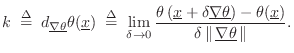
Scattering of plane waves is discussed in §C.8.1.
Solving the 2D Wave Equation
Since solving the wave equation in 2D has all the essential features of the 3D case, we will look at the 2D case in this section.
Specializing Eq.![]() (B.47) to 2D, the 2D wave equation may
be written as
(B.47) to 2D, the 2D wave equation may
be written as
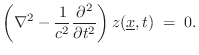
The 2D wave equation is obeyed by traveling sinusoidal plane
waves having any amplitude ![]() , radian frequency
, radian frequency ![]() , phase
, phase
![]() , and direction
, and direction
![]() :
:
The sum of two such waves traveling in opposite directions with the
same amplitude and frequency produces a standing wave. For example,
if the waves are traveling parallel to the ![]() axis, we have
axis, we have
which is a standing wave along
2D Boundary Conditions
We often wish to find solutions of the 2D wave equation that obey
certain known boundary conditions. An example is transverse
waves on an ideal elastic membrane, rigidly clamped on its boundary to
form a rectangle with dimensions ![]() meters.
meters.
Similar to the derivation of Eq.![]() (B.49), we can subtract
the second sinusoidal traveling wave from the first to yield
(B.49), we can subtract
the second sinusoidal traveling wave from the first to yield
Note that we can also use products of horizontal and vertical standing waves
To build solutions to the wave equation that obey all of the boundary conditions, we can form linear combinations of the above standing-wave products having zero displacement (``nodes'') along all four boundary lines:
where
The Wikipedia page (as of 1/31/10) on the Helmholtz equation provides a nice ``entry point'' on the above topics and further information.
3D Sound
The mathematics of 3D sound is quite elementary, as we will see below. The hard part of the theory of practical systems typically lies in the mathematical approximation to the ideal case. Examples include Ambisonics [158] and wave field synthesis [49].
Consider a point source at position
![]() . Then the
acoustic complex amplitude at position
. Then the
acoustic complex amplitude at position
![]() is given by
is given by

The fundamental approximation problem in 3D sound is to approximate
the complex acoustic field at one or more listening points using a
finite set of ![]() loudspeakers, which are often modeled as a point
source for each speaker.
loudspeakers, which are often modeled as a point
source for each speaker.
Next Section:
Digital Waveguide Theory
Previous Section:
A History of Enabling Ideas Leading to Virtual Musical Instruments


