Feedforward Comb Filters

The feedforward comb filter is shown in Fig.2.23. The direct signal ``feeds forward'' around the delay line. The output is a linear combination of the direct and delayed signal.

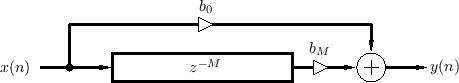
The ``difference equation'' [449] for the feedforward comb filter is

We see that the feedforward comb filter is a particular type of FIR filter. It is also a special case of a TDL.

Note that the feedforward comb filter can implement the echo simulator of Fig.2.9 by setting and . Thus, it is is a computational physical model of a single discrete echo. This is one of the simplest examples of acoustic modeling using signal processing elements. The feedforward comb filter models the superposition of a ``direct signal'' plus an attenuated, delayed signal , where the attenuation (by ) is due to ``air absorption'' and/or spherical spreading losses, and the delay is due to acoustic propagation over the distance meters, where is the sampling period in seconds, and is sound speed. In cases where the simulated propagation delay needs to be more accurate than the nearest integer number of samples , some kind of delay-line interpolation needs to be used (the subject of §4.1). Similarly, when air absorption needs to be simulated more accurately, the constant attenuation factor can be replaced by a linear, time-invariant filter giving a different attenuation at every frequency. Due to the physics of air absorption, is generally lowpass in character [349, p. 560], [47,318].

---

Previous: Comb Filters
Next: Feedback Comb Filters

Order a Hardcopy of Physical Audio Signal Processing

---

About the Author: Julius Orion Smith III
Julius Smith's background is in electrical engineering (BS Rice 1975, PhD Stanford 1983). He is presently Professor of Music and Associate Professor (by courtesy) of Electrical Engineering at Stanford's Center for Computer Research in Music and Acoustics (CCRMA), teaching courses and pursuing research related to signal processing applied to music and audio systems. See http://ccrma.stanford.edu/~jos/ for details.