


The Finite Difference Approximation
In the musical acoustics literature, the normal method for creating a computational model from a differential equation is to apply the so-called finite difference approximation (FDA) in which differentiation is replaced by a finite difference (see Appendix D) [481,311]. For example
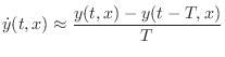
and
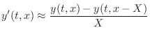
where
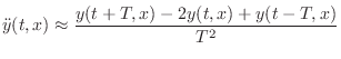

The odd-order derivative approximations suffer a half-sample delay error while all even order cases can be compensated as above.
FDA of the Ideal String
Substituting the FDA into the wave equation gives

![$\displaystyle \frac{KT^2}{\epsilon X^2}
\left[ y(t,x+X) - 2 y(t,x) + y(t,x-X)\right]$](http://www.dsprelated.com/josimages_new/pasp/img3213.png)
In a practical implementation, it is common to set
Thus, to update the sampled string displacement, past values are needed for each point along the string at time instants
Perhaps surprisingly, it is shown in Appendix E that the above recursion is exact at the sample points in spite of the apparent crudeness of the finite difference approximation [442]. The FDA approach to numerical simulation was used by Pierre Ruiz in his work on vibrating strings [392], and it is still in use today [74,75].
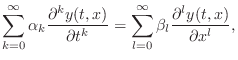
When more terms are added to the wave equation, corresponding to complex
losses and dispersion characteristics, more terms of the form
![]() appear in (C.6). These higher-order terms correspond to
frequency-dependent losses and/or dispersion characteristics in
the FDA. All linear differential equations with constant coefficients give rise to
some linear, time-invariant discrete-time system via the FDA.
A general subclass of the linear, time-invariant case
giving rise to ``filtered waveguides'' is
appear in (C.6). These higher-order terms correspond to
frequency-dependent losses and/or dispersion characteristics in
the FDA. All linear differential equations with constant coefficients give rise to
some linear, time-invariant discrete-time system via the FDA.
A general subclass of the linear, time-invariant case
giving rise to ``filtered waveguides'' is
 |
(C.7) |
while the fully general linear, time-invariant 2D case is
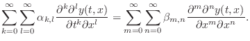 |
(C.8) |
A nonlinear example is
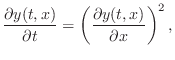 |
(C.9) |
and a time-varying example can be given by
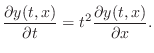 |
(C.10) |
Next Section:
Traveling-Wave Solution
Previous Section:
The Ideal Vibrating String


