


High-Accuracy Piano-String Modeling
In [265,266], an extension of the mass-spring model of [391] was presented for the purpose of high-accuracy modeling of nonlinear piano strings struck by a hammer model such as described in §9.3.2. This section provides a brief overview.
![\includegraphics[width=0.35\twidth]{eps/massspringmass}](http://www.dsprelated.com/josimages_new/pasp/img2271.png)
Figure 9.25 shows a mass-spring model in 3D space. From Hooke's Law (§B.1.3), we have
![\begin{eqnarray*}
m_1\, \underline{{\ddot x}}_1 \eqsp \underline{f}_1
&=& k\cdo...
...,\right\Vert}\right]\left(\underline{x}_2-\underline{x}_1\right)
\end{eqnarray*}](http://www.dsprelated.com/josimages_new/pasp/img2276.png)
and similarly for mass 2, where
![]() is the vector
position of mass
is the vector
position of mass ![]() in 3D space.
in 3D space.
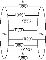
Generalizing to a chain of masses and spring is shown in Fig.9.26. Mass-spring chains--also called beaded strings--have been analyzed in numerous textbooks (e.g., [295,318]), and numerical software simulation is described in [391].
![\includegraphics[width=0.8\twidth]{eps/massspringstring}](http://www.dsprelated.com/josimages_new/pasp/img2278.png)
The force on the ![]() th mass can be expressed as
th mass can be expressed as
where
![$\displaystyle \alpha_i \isdefs k\cdot \left[1-\frac{l_0}{\left\Vert\,\underline{x}_{i+1}-\underline{x}_i\,\right\Vert}\right].
$](http://www.dsprelated.com/josimages_new/pasp/img2282.png)
A Stiff Mass-Spring String Model
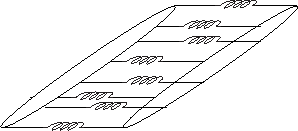
Following the classical derivation of the stiff-string wave equation [317,144], an obvious way to introduce stiffness in the mass-spring chain is to use a bundle of mass-spring chains to form a kind of ``lumped stranded cable''. One section of such a model is shown in Fig.9.27. Each mass is now modeled as a 2D mass disk. Complicated rotational dynamics can be avoided by assuming no torsional waves (no ``twisting'' motion) (§B.4.20).
A three-spring-per-mass model is shown in Fig.9.28
[266]. The spring positions alternate between angles
![]() , say, on one side of a mass disk and
, say, on one side of a mass disk and
![]() on the other side in order to provide effectively
six spring-connection points around the mass disk for only
three connecting springs per section. This improves isotropy
of the string model with respect to bending direction.
on the other side in order to provide effectively
six spring-connection points around the mass disk for only
three connecting springs per section. This improves isotropy
of the string model with respect to bending direction.
![\includegraphics[width=0.8\twidth]{eps/masssprings3circ}](http://www.dsprelated.com/josimages_new/pasp/img2286.png)
A problem with the simple mass-spring-chain-bundle is that there is no
resistance whatsoever to shear deformation, as is clear from
Fig.9.29. To rectify this problem (which does not
arise due implicit assumptions when classically deriving the
stiff-string wave equation), diagonal springs can be added to the
model, as shown in
Fig.![]() .
.
In the simulation results reported in [266], the spring-constants of the shear springs were chosen so that their stiffness in the longitudinal direction would equal that of the longitudinal springs.
![\includegraphics[width=0.4\twidth]{eps/masssprings3shear}](http://www.dsprelated.com/josimages_new/pasp/img2288.png)
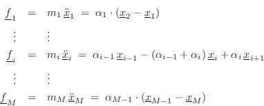
Nonlinear Piano-String Equations of Motion in State-Space Form
For the flexible (non-stiff) mass-spring string, referring to
Fig.9.26 and Eq.![]() (9.34), we have the following
equations of motion:
(9.34), we have the following
equations of motion:
or, in ![]() vector form,
vector form,
Finite Difference Implementation
Digitizing
![]() via the centered second-order difference
[Eq.
via the centered second-order difference
[Eq.![]() (7.5)]
(7.5)]
Note that requiring three adjacent spatial string samples to be in
contact with the piano hammer during the attack (which helps to
suppress aliasing of spatial frequencies on the string during the
attack) implies a sampling rate in the vicinity of 6 megahertz
[265]. Thus, the model is expensive to compute!
However, results to date show a high degree of accuracy, as desired.
In particular, the stretching of the partial overtones in the
stiff-string model of
Fig.![]() has
been measured to be highly accurate despite using only three spring
attachment points on one side of each mass disk [265].
has
been measured to be highly accurate despite using only three spring
attachment points on one side of each mass disk [265].
See [53] for alternative finite-difference formulations that better preserve physical energy and have other nice properties worth considering.
Next Section:
Commuted Piano Synthesis
Previous Section:
Nonlinear Piano Strings


