


Impulse Invariant Method
The impulse-invariant method converts analog filter transfer
functions to digital filter transfer functions in such a way that the
impulse response is the same (invariant) at the sampling
instants [343], [362, pp.
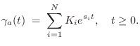
216-219]. Thus, if ![]() denotes the
impulse-response of an analog (continuous-time) filter, then the
digital (discrete-time) filter given by the impulse-invariant method
will have impulse response
denotes the
impulse-response of an analog (continuous-time) filter, then the
digital (discrete-time) filter given by the impulse-invariant method
will have impulse response
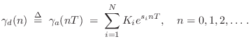
![]() , where
, where ![]() denotes the
sampling interval in seconds. Moreover, the order of the filter is
preserved, and IIR analog filters map to IIR digital filters.
However, the digital filter's frequency response is an aliased
version of the analog filter's frequency
response.9.3
denotes the
sampling interval in seconds. Moreover, the order of the filter is
preserved, and IIR analog filters map to IIR digital filters.
However, the digital filter's frequency response is an aliased
version of the analog filter's frequency
response.9.3
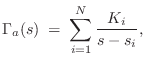
To derive the impulse-invariant method, we begin with the analog transfer function

and perform a partial fraction expansion (PFE) down to first-order terms [449]:9.4
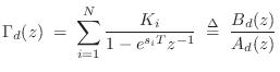

and the residues have remained unchanged. Clearly we must have
Note that the series combination of two digital filters designed by the impulse-invariant method is not impulse invariant. In other terms, the convolution of two sampled analog signals is not the same as the sampled convolution of those analog signals. This is easy to see when aliasing is considered. For example, let one signal be the impulse response of an ideal lowpass filter cutting off below half the sampling rate. Then this signal will not alias when sampled, and its convolution with any second signal will similarly not alias when sampled. However, if the second signal does alias upon sampling, then this aliasing is gone when the convolution precedes the sampling, and the results cannot be the same in the two cases.
Next Section:
Matched Z Transformation
Previous Section:
Sampling the Impulse Response


