Sign in

Search Online Books

Free Online Books

Sponsor

Industry's highest performing at the lowest power DSPs now as low as $5.00*
Start development today!
*volume pricing for 10ku

Chapters

Physical Audio Signal Processing
    Elementary Physics, Mechanics, and Acoustics
       Rigid-Body Dynamics
          Mass Moment of Inertia Tensor

Chapter Contents:

Search Physical Audio Signal Processing

Book Index | Global Index

Would you like to be notified by email when Julius Orion Smith III publishes a new entry into his blog?

Mass Moment of Inertia Tensor

As derived in the previous section, the moment of inertia tensor, in 3D Cartesian coordinates, is a three-by-three matrix $\mathbf{I}$ that can be multiplied by any angular-velocity vector to produce the corresponding angular momentum vector for either a point mass or a rigid mass distribution. Note that the origin of the angular-velocity vector $\underline{\omega}$ is always fixed at $\underline{0}$ in the space (typically located at the center of mass). Therefore, the moment of inertia tensor $\mathbf{I}$ is defined relative to that origin.

The moment of inertia tensor can similarly be used to compute the mass moment of inertia for any normalized angular velocity vector $\underline{\tilde{\omega}}=\underline{\omega}/ \vert\vert\,\underline{\omega}\,\vert\vert$ as

$\displaystyle I \eqsp \underline{\tilde{\omega}}^T\mathbf{I}\,\underline{\tilde{\omega}}. \protect$

(B.22)

Since rotational energy is defined as $(1/2)I\omega^2$ (see Eq. $\,$ (B.7)), multiplying Eq. $\,$ (B.22) by $\omega^2$ gives the following expression for the rotational kinetic energy in terms of the moment of inertia tensor:

$\displaystyle E_R \eqsp \frac{1}{2}\, \underline{\omega}^T\mathbf{I}\,\underline{\omega} \protect$

(B.23)

We can show Eq. $\,$ (B.22) starting from Eq. $\,$ (B.14). For a point-mass

located at $\underline{x}$ , we have

$\begin{eqnarray*} I &=& m \left\Vert\,\underline{x}-(\underline{\tilde{\omega}}^... ...nderline{\tilde{\omega}}^T\mathbf{I}\,\underline{\tilde{\omega}} \end{eqnarray*}$

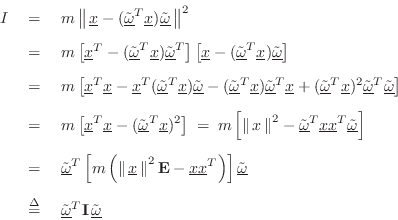
where again $\mathbf{E}$ denotes the three-by-three identity matrix, and

$\displaystyle \mathbf{I}\eqsp m \left(\left\Vert\,\underline{x}\,\right\Vert^2\mathbf{E}-\underline{x}\underline{x}^T\right), \protect$

(B.24)

which agrees with Eq. $\,$ (B.20). Thus we have derived the moment of inertia

in terms of the moment of inertia tensor $\mathbf{I}$ and the normalized angular velocity $\underline{\tilde{\omega}}$ for a point-mass

at $\underline{x}$ .

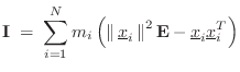
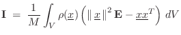
For a collection of masses located at $\underline{x}_i\in{\bf R}^3$ , we simply sum over their masses to add up the moments of inertia:

$\displaystyle \mathbf{I}\eqsp \sum_{i=1}^N m_i \left(\left\Vert\,\underline{x}_i\,\right\Vert^2\mathbf{E} -\underline{x}_i\underline{x}_i^T\right)$

Finally, for a continuous mass distribution, we integrate as usual:

$\displaystyle \mathbf{I}\eqsp \frac{1}{M}\int_V \rho(\underline{x}) \left(\left... ...underline{x}\,\right\Vert^2\mathbf{E} -\underline{x}\underline{x}^T\right)\,dV$

where $M=\int_V\rho(\underline{x})dV$ is the total mass.

Subsections

Previous: Angular Momentum Vector in Matrix Form
Next: Simple Example

Order a Hardcopy of Physical Audio Signal Processing

About the Author: Julius Orion Smith III
Julius Smith's background is in electrical engineering (BS Rice 1975, PhD Stanford 1983). He is presently Professor of Music and Associate Professor (by courtesy) of Electrical Engineering at Stanford's Center for Computer Research in Music and Acoustics (CCRMA), teaching courses and pursuing research related to signal processing applied to music and audio systems. See http://ccrma.stanford.edu/~jos/ for details.

Comments

No comments yet for this page

Add a Comment

You need to login before you can post a comment (best way to prevent spam). ( Not a member? )