


A More Formal Derivation of the Wave Digital Force-Driven Mass
Above we derived how to handle the external force by direct physical reasoning. In this section, we'll derive it using a more general step-by-step procedure which can be applied systematically to more complicated situations.
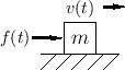
Figure F.10 gives the physical picture of a free mass driven by
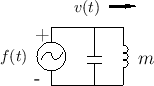
an external force in one dimension. Figure F.11 shows the
electrical equivalent circuit for this scenario in which the external
force is represented by a voltage source emitting ![]() volts,
and the mass is modeled by an inductor having the value
volts,
and the mass is modeled by an inductor having the value ![]() Henrys.
Henrys.
 |
The next step is to convert the voltages and currents in the
electrical equivalent circuit to wave variables.
Figure F.12 gives an intermediate equivalent circuit in which
an infinitesimal transmission line section with real impedance ![]() has been inserted to facilitate the computation of the wave-variable
reflectance, as we did in §F.1.1 to derive Eq.
has been inserted to facilitate the computation of the wave-variable
reflectance, as we did in §F.1.1 to derive Eq.![]() (F.1).
(F.1).
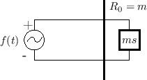 |
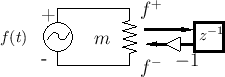
Figure F.13 depicts a next intermediate equivalent circuit in
which the mass has been replaced by its reflectance (using ``![]() ''
to denote the continuous-time reflectance
''
to denote the continuous-time reflectance
![]() , as derived in
§F.1.1). The infinitesimal transmission-line section is now represented
by a ``resistor'' since, when the voltage source is initially
``switched on'', it only ``sees'' a real resistance having the value
, as derived in
§F.1.1). The infinitesimal transmission-line section is now represented
by a ``resistor'' since, when the voltage source is initially
``switched on'', it only ``sees'' a real resistance having the value
![]() Ohms (the waveguide interface). After a short period of time
determined by the reflectance of the mass,F.4 ``return waves'' from the mass result in an ultimately
reactive impedance. This of course must be the case because the
mass does not dissipate energy. Therefore, the ``resistor'' of
Ohms (the waveguide interface). After a short period of time
determined by the reflectance of the mass,F.4 ``return waves'' from the mass result in an ultimately
reactive impedance. This of course must be the case because the
mass does not dissipate energy. Therefore, the ``resistor'' of ![]() Ohms is not a resistor in the usual sense since it does not convert
potential energy (the voltage drop across it) into heat. Instead, it
converts potential energy into propagating waves with 100%
efficiency. Since all of this wave energy is ultimately reflected by
the terminating element (mass, spring, or any combination of masses
and springs), the net effect is a purely reactive impedance, as we
know it must be.
Ohms is not a resistor in the usual sense since it does not convert
potential energy (the voltage drop across it) into heat. Instead, it
converts potential energy into propagating waves with 100%
efficiency. Since all of this wave energy is ultimately reflected by
the terminating element (mass, spring, or any combination of masses
and springs), the net effect is a purely reactive impedance, as we
know it must be.
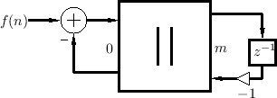 |
To complete the wave digital model, we need to connect our wave
digital mass to an ideal force source which asserts the value ![]() each sample time. Since an ideal force source has a zero internal
impedance, we desire a parallel two-port junction which connects the
impedances
each sample time. Since an ideal force source has a zero internal
impedance, we desire a parallel two-port junction which connects the
impedances ![]() (
(
![]() ) and
) and ![]() (
(
![]() ), as
shown in Fig.F.14. From
Eq.
), as
shown in Fig.F.14. From
Eq.![]() (F.18) we have that the common junction force is equal to
(F.18) we have that the common junction force is equal to
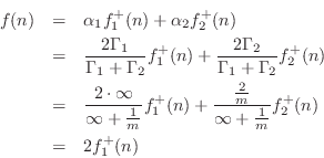
from which we conclude that

Since
![]() and
and
![]() for this model, the reflection
coefficient seen on port 1 is
for this model, the reflection
coefficient seen on port 1 is
![]() . The
transmission coefficient from port 1 is
. The
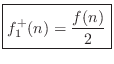
transmission coefficient from port 1 is ![]() . In the opposite
direction, the reflection coefficient on port 2 is
. In the opposite
direction, the reflection coefficient on port 2 is ![]() , and
the transmission coefficient from port 2 is
, and
the transmission coefficient from port 2 is
![]() . The final
result, drawn in Kelly-Lochbaum form (see §F.2.1), is
diagrammed in Fig.F.15, as well as the result of some
elementary simplifications. The final model is the same as in
Fig.F.9, as it should be.
. The final
result, drawn in Kelly-Lochbaum form (see §F.2.1), is
diagrammed in Fig.F.15, as well as the result of some
elementary simplifications. The final model is the same as in
Fig.F.9, as it should be.
Next Section:
Checking the WDF against the Analog Equivalent Circuit
Previous Section:
Extracting Physical Quantities


