


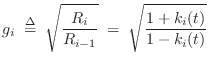
Normalized Scattering Junctions
![\includegraphics[scale=0.9]{eps/scatnlf}](http://www.dsprelated.com/josimages_new/pasp/img3623.png)
Using (C.53) to convert to normalized waves
![]() , the
Kelly-Lochbaum junction (C.60) becomes
, the
Kelly-Lochbaum junction (C.60) becomes
as diagrammed in Fig.C.22. This is called the normalized scattering junction [297], although a more precise term would be the ``normalized-wave scattering junction.''
It is interesting to define
![]() , always
possible for passive junctions since
, always
possible for passive junctions since
![]() , and note that
the normalized scattering junction is equivalent to a 2D rotation:
, and note that
the normalized scattering junction is equivalent to a 2D rotation:
where, for conciseness of notation, the time-invariant case is written.
While it appears that scattering of normalized waves at a two-port junction requires four multiplies and two additions, it is possible to convert this to three multiplies and three additions using a two-multiply ``transformer'' to power-normalize an ordinary one-multiply junction [432].
The transformer is a lossless two-port defined by [136]
The transformer can be thought of as a device which steps the wave impedance to a new value without scattering; instead, the traveling signal power is redistributed among the force and velocity wave variables to satisfy the fundamental relations
as can be quickly derived by requiring
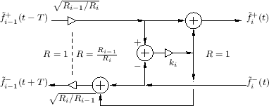
Figure C.23 illustrates a three-multiply
normalized-wave scattering junction [432]. The impedance of
all waveguides (bidirectional delay lines) may be taken to be ![]() .
Scattering junctions may then be implemented as a denormalizing
transformer
.
Scattering junctions may then be implemented as a denormalizing
transformer
![]() , a one-multiply scattering junction
, a one-multiply scattering junction
![]() , and a renormalizing transformer
, and a renormalizing transformer
![]() . Either
transformer may be commuted with the junction and combined with the
other transformer to give a three-multiply normalized-wave scattering
junction. (The transformers are combined on the left in
Fig.C.23).
. Either
transformer may be commuted with the junction and combined with the
other transformer to give a three-multiply normalized-wave scattering
junction. (The transformers are combined on the left in
Fig.C.23).
In slightly more detail, a transformer
![]() steps the wave
impedance (left-to-right) from
steps the wave
impedance (left-to-right) from ![]() to
to ![]() . Equivalently, the
normalized force-wave
. Equivalently, the
normalized force-wave
![]() is converted unnormalized form
is converted unnormalized form
![]() . Next there is a physical scattering from impedance
. Next there is a physical scattering from impedance
![]() to
to ![]() (reflection coefficient
(reflection coefficient
![]() ). The outgoing wave to the right is
then normalized by transformer
). The outgoing wave to the right is
then normalized by transformer
![]() to return the wave
impedance back to
to return the wave
impedance back to ![]() for wave propagation within a normalized-wave
delay line to the right. Finally, the right transformer is commuted
left and combined with the left transformer to reduce total
computational complexity to one multiply and three adds.
for wave propagation within a normalized-wave
delay line to the right. Finally, the right transformer is commuted
left and combined with the left transformer to reduce total
computational complexity to one multiply and three adds.
It is important to notice that transformer-normalized junctions may
have a large dynamic range in practice. For example, if
![]() , then Eq.
, then Eq.![]() (C.69) shows that the
transformer coefficients may become as large as
(C.69) shows that the
transformer coefficients may become as large as
![]() . If
. If ![]() is the ``machine epsilon,'' i.e.,
is the ``machine epsilon,'' i.e.,
![]() for typical
for typical ![]() -bit two's complement arithmetic normalized
to lie in
-bit two's complement arithmetic normalized
to lie in ![]() , then the dynamic range of the transformer
coefficients is bounded by
, then the dynamic range of the transformer
coefficients is bounded by
![]() . Thus, while
transformer-normalized junctions trade a multiply for an add, they
require up to
. Thus, while
transformer-normalized junctions trade a multiply for an add, they
require up to ![]() % more bits of dynamic range within the junction
adders. On the other hand, it is very nice to have normalized waves
(unit wave impedance) throughout the digital waveguide network,
thereby limiting the required dynamic range to root physical power in
all propagation paths.
% more bits of dynamic range within the junction
adders. On the other hand, it is very nice to have normalized waves
(unit wave impedance) throughout the digital waveguide network,
thereby limiting the required dynamic range to root physical power in
all propagation paths.
Next Section:
Junction Passivity
Previous Section:
One-Multiply Scattering Junctions


