


Rotating Horn Simulation
The heart of the Leslie effect is a rotating horn loudspeaker. The rotating horn from a Model 600 Leslie can be seen mounted on a microphone stand in Fig.5.7. Two horns are apparent, but one is a dummy, serving mainly to cancel the centrifugal force of the other during rotation. The Model 44W horn is identical to that of the Model 600, and evidently standard across all Leslie models [189]. For a circularly rotating horn, the source position can be approximated as
![$\displaystyle \underline{x}_s(t) = \left[\begin{array}{c} r_s\cos(\omega_m t) \\ [2pt] r_s\sin(\omega_m t) \end{array}\right] \protect$](http://www.dsprelated.com/josimages_new/pasp/img1293.png)
where
By Eq.
![\includegraphics[width=4.1in]{eps/hornrecordingr}](http://www.dsprelated.com/josimages_new/pasp/img1296.png)
![$\displaystyle \underline{v}_s(t) = \frac{d}{dt}\underline{x}_s(t) = \left[\begi...
...in(\omega_m t) \\ [2pt] r_s\omega_m\cos(\omega_m t) \end{array}\right] \protect$](http://www.dsprelated.com/josimages_new/pasp/img1297.png)
Note that the source velocity vector is always orthogonal to the source position vector, as indicated in Fig.5.8.
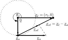
Since
![]() and
and
![]() are orthogonal,
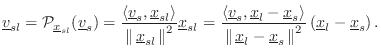
the projected source velocity Eq.
are orthogonal,
the projected source velocity Eq.![]() (5.4) simplifies to
(5.4) simplifies to
Arbitrarily choosing
![$\displaystyle \underline{v}_{sl}= \frac{-r_l r_s\omega_m\sin(\omega_m t)}{r_l^2...
...l-r_s\cos(\omega_m t) \\ [2pt] -r_s\sin(\omega_m)t \end{array}\right]. \protect$](http://www.dsprelated.com/josimages_new/pasp/img1302.png)
In the far field, this reduces simply to
![$\displaystyle \underline{v}_{sl}\approx -r_s\omega_m\sin(\omega_m t) \left[\begin{array}{c} 1 \\ [2pt] 0 \end{array}\right]. \protect$](http://www.dsprelated.com/josimages_new/pasp/img1303.png)
Substituting into the Doppler expression Eq.
where the approximation is valid for small Doppler shifts. Thus, in the far field, a rotating horn causes an approximately sinusoidal multiplicative frequency shift, with the amplitude given by horn length
Next Section:
Rotating Woofer-Port and Cabinet
Previous Section:
System Block Diagram


