


State-Space Analysis
We will now use state-space analysisC.15[449] to determine Equations (C.133-C.136).
![$\displaystyle \left[\begin{array}{c} x_1(n+1) \\ [2pt] x_2(n+1) \end{array}\rig...
...bf{A} \left[\begin{array}{c} x_1(n) \\ [2pt] x_2(n) \end{array}\right] \protect$](http://www.dsprelated.com/josimages_new/pasp/img4193.png)
or, in vector notation,
| (C.137) | |||
| (C.138) |
where we have introduced an input signal
A basic fact from linear algebra is that the determinant of a
matrix is equal to the product of its eigenvalues. As a quick
check, we find that the determinant of ![]() is
is
When the eigenvalues
Note that
![]() . If we diagonalize this system to
obtain
. If we diagonalize this system to
obtain
![]() , where
, where
![]() diag
diag![]() , and
, and
![]() is the matrix of eigenvectors
of
is the matrix of eigenvectors
of
![]() , then we have
, then we have
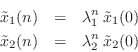
![$\displaystyle \tilde{\underline{x}}(n) = \tilde{A}^n\,\tilde{\underline{x}}(0) ...
...eft[\begin{array}{c} \tilde{x}_1(0) \\ [2pt] \tilde{x}_2(0) \end{array}\right]
$](http://www.dsprelated.com/josimages_new/pasp/img4209.png)
If this system is to generate a real sampled sinusoid at radian frequency
![]() , the eigenvalues
, the eigenvalues ![]() and
and ![]() must be of the form
must be of the form
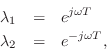
(in either order) where ![]() is real, and
is real, and ![]() denotes the sampling
interval in seconds.
denotes the sampling
interval in seconds.
Thus, we can determine the frequency of oscillation ![]() (and
verify that the system actually oscillates) by determining the
eigenvalues
(and
verify that the system actually oscillates) by determining the
eigenvalues ![]() of
of ![]() . Note that, as a prerequisite, it will
also be necessary to find two linearly independent eigenvectors of
. Note that, as a prerequisite, it will
also be necessary to find two linearly independent eigenvectors of ![]() (columns of
(columns of
![]() ).
).
Next Section:
Eigenstructure
Previous Section:
Digital Waveguide Resonator


