


State Transformations
In previous work, time-domain adaptors (digital filters) converting
between K variables and W variables have been devised
[223]. In this section, an alternative approach is
proposed. Mapping Eq.![]() (E.7) gives us an immediate conversion from W
to K state variables, so all we need now is the inverse map for any
time
(E.7) gives us an immediate conversion from W
to K state variables, so all we need now is the inverse map for any
time ![]() . This is complicated by the fact that non-local spatial
dependencies can go indefinitely in one direction along the string, as
we will see below. We will proceed by first writing down the
conversion from W to K variables in matrix form, which is easy to do,
and then invert that matrix. For simplicity, we will consider the
case of an infinitely long string.
. This is complicated by the fact that non-local spatial
dependencies can go indefinitely in one direction along the string, as
we will see below. We will proceed by first writing down the
conversion from W to K variables in matrix form, which is easy to do,
and then invert that matrix. For simplicity, we will consider the
case of an infinitely long string.
To initialize a K variable simulation for starting at time ![]() , we
need initial spatial samples at all positions
, we
need initial spatial samples at all positions ![]() for two successive
times
for two successive
times ![]() and
and ![]() . From this state specification, the FDTD scheme
Eq.
. From this state specification, the FDTD scheme
Eq.![]() (E.3) can compute
(E.3) can compute ![]() for all
for all ![]() , and so on for
increasing
, and so on for
increasing ![]() . In the DW model, all state variables are defined as
belonging to the same time
. In the DW model, all state variables are defined as
belonging to the same time ![]() , as shown in Fig.E.2.
, as shown in Fig.E.2.
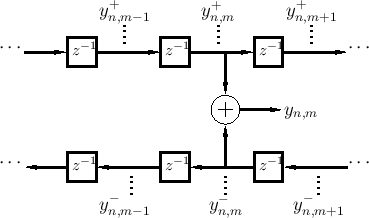
From Eq.![]() (E.6), and referring to the notation defined in
Fig.E.2, we may write the conversion from W to K variables
as
(E.6), and referring to the notation defined in
Fig.E.2, we may write the conversion from W to K variables
as
where the last equality follows from the traveling-wave behavior (see Fig.E.2).
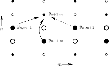
Figure E.3 shows the so-called ``stencil'' of the FDTD scheme.
The larger circles indicate the state at time ![]() which can be used to
compute the state at time
which can be used to
compute the state at time ![]() . The filled and unfilled circles
indicate membership in one of two interleaved grids [55]. To
see why there are two interleaved grids, note that when
. The filled and unfilled circles
indicate membership in one of two interleaved grids [55]. To
see why there are two interleaved grids, note that when ![]() is even,
the update for
is even,
the update for ![]() depends only on odd
depends only on odd ![]() from time
from time ![]() and even
and even
![]() from time
from time ![]() . Since the two W components of
. Since the two W components of ![]() are converted to
two W components at time
are converted to
two W components at time ![]() in Eq.
in Eq.![]() (E.8), we have that the update for
(E.8), we have that the update for
![]() depends only on W components from time
depends only on W components from time ![]() and positions
and positions
![]() .
Moving to the next position update, for
.
Moving to the next position update, for
![]() , the state used is
independent of that used for
, the state used is
independent of that used for ![]() , and the W components used are
from positions
, and the W components used are
from positions ![]() and
and ![]() . As a result of these observations, we
see that we may write the state-variable transformation separately for
even and odd
. As a result of these observations, we
see that we may write the state-variable transformation separately for
even and odd ![]() , e.g.,
, e.g.,
![$\displaystyle \left[\! \begin{array}{c} \vdots \\ y_{n,m-1}\\ y_{n-1,m}\\ y_{n,...
...n,m+3}\\ y^{+}_{n,m+5}\\ y^{-}_{n,m+5}\\ \vdots \end{array} \!\right]. \protect$](http://www.dsprelated.com/josimages_new/pasp/img4535.png)
Denote the linear transformation operator by
The operator
![$\displaystyle \left[\! \begin{array}{c} \vdots \\ y^{+}_{n,m-1}\\ y^{-}_{n,m-1}...
... y_{n,m+3}\\ y_{n-1,m+4}\\ y_{n,m+5}\\ \vdots \\ \end{array} \!\right] \protect$](http://www.dsprelated.com/josimages_new/pasp/img4542.png)
The case of the finite string is identical to that of the infinite string when the matrix
Next Section:
Excitation Examples
Previous Section:
Introduction


