Sign in

Search Online Books

Free Online Books

Sponsor

Industry's highest performing at the lowest power DSPs now as low as $5.00*
Start development today!
*volume pricing for 10ku

Chapters

Physical Audio Signal Processing
    Virtual Musical Instruments
       String Excitation
          Ideal String Struck by a Mass
             Summary of Mass-String Scattering Junction

Chapter Contents:

Search Physical Audio Signal Processing

Book Index | Global Index

Would you like to be notified by email when Julius Orion Smith III publishes a new entry into his blog?

Summary of Mass-String Scattering Junction

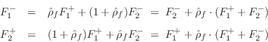
In summary, we have characterized the mass on the string in terms of its reflectance and transmittance from either string. For force waves, we have outgoing waves given by

$\begin{eqnarray*} F^{-}_1(s) &=& \hat{\rho}_f(s) F^{+}_1(s) + \hat{\tau}_f(s) F^... ...2(s) &=& \hat{\tau}_f(s) F^{+}_1(s) + \hat{\rho}_f(s) F^{-}_2(s) \end{eqnarray*}$

$\displaystyle \left[\begin{array}{c} F^{+}_2 \\ [2pt] F^{-}_1 \end{array}\right... ...ay}\right] \left[\begin{array}{c} F^{+}_1 \\ [2pt] F^{-}_2 \end{array}\right]$

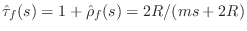
in terms of the incoming waves $F^{+}_1$ and $F^{-}_2$ , the force reflectance $\hat{\rho}_f(s)=ms/(ms+2R)$ , and the force transmittance $\hat{\tau}_f(s)=1+\hat{\rho}_f(s)=2R/(ms+2R)$ . We may say that the mass creates a dynamic scattering junction on the string. (If there were no dependency on

, such as when a dashpot is affixed to the string, we would simply call it a scattering junction.) The above form of the dynamic scattering junction is analogous to the Kelly-Lochbaum scattering junction (§C.8.4). The general relation $\hat{\tau}_f = 1+\hat{\rho}_f$ can be used to simplify the Kelly-Lochbaum form to a one-filter scattering junction analogous to the one-multiply scattering junction (§C.8.5):

$\begin{eqnarray*} F^{-}_1 &=& \hat{\rho}_f F^{+}_1 + (1+\hat{\rho}_f) F^{-}_2 \;... ...ho}_f F^{-}_2 \;=\; F^{+}_1 + \hat{\rho}_f\cdot(F^{+}_1+F^{-}_2) \end{eqnarray*}$

The one-filter form follows from the observation that $\hat{\rho}_f\cdot(F^{+}_1+F^{-}_2)$ appears in both computations, and therefore need only be implemented once:

$\begin{eqnarray*} F^{+}&\isdef & \hat{\rho}_f\cdot(F^{+}_1+F^{-}_2)\\ [5pt] F^{-}_1 &=& F^{-}_2 + F^{+}\\ [5pt] F^{+}_2 &=& F^{+}_1 + F^{+} \end{eqnarray*}$

This structure is diagrammed in Fig.9.20.

**Figure 9.20:** Continuous-time force-wave simulation diagram, in one-filter form, for an ideal string with a point mass attached.
$\includegraphics[width=\twidth]{eps/massstringdwms}$

Again, the above results follow immediately from the more general formulation of §C.12.

Previous: Force Wave Mass-String Model
Next: Digital Waveguide Mass-String Model

Order a Hardcopy of Physical Audio Signal Processing

About the Author: Julius Orion Smith III
Julius Smith's background is in electrical engineering (BS Rice 1975, PhD Stanford 1983). He is presently Professor of Music and Associate Professor (by courtesy) of Electrical Engineering at Stanford's Center for Computer Research in Music and Acoustics (CCRMA), teaching courses and pursuing research related to signal processing applied to music and audio systems. See http://ccrma.stanford.edu/~jos/ for details.

Comments

No comments yet for this page

Add a Comment

You need to login before you can post a comment (best way to prevent spam). ( Not a member? )