Free Books Physical Audio Signal Processing

Transfer Function Models

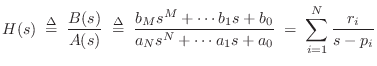
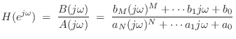
For linear time-invariant systems, rather than build an explicit discrete-time model as in §7.3 for each mass, spring, and dashpot, (or inductor, capacitor, and resistor for virtual analog models), we may instead choose to model only the transfer function between selected inputs and outputs of the physical system. It should be emphasized that this is an option only when the relevant portion of the system is linear and time invariant (LTI), or at least sufficiently close to LTI. Transfer-function modeling can be considered a kind of ``large-scale'' or ``macroscopic'' modeling in which an entire physical subsystem, such as a guitar body, is modeled by a single transfer function relating specific inputs and outputs. (A transfer function can also of course be a matrix relating a vector of inputs to a vector of outputs [220].) Such models are used extensively in the field of control system design [150].^9.1

Transfer-function modeling is often the most cost-effective way to incorporate LTI lumped elements (Ch. 7) in an otherwise physical computational model. For wave-propagating distributed systems, on the other hand, such as vibrating strings and acoustic tubes, digital waveguides models (Ch. 6) are more efficient than transfer-function models, in addition to having a precise physical interpretation that transfer-function coefficients lack. In models containing lumped elements, or distributed components that are not characterized by wave propagation, maximum computational efficiency is typically obtained by deciding which LTI portions of the model can be ``frozen'' as ``black boxes'' characterized only by their transfer functions. In return for increased computational efficiency, we sacrifice the ability to access the interior of the black box in a physically meaningful way.

An example where such ``macroscopic'' transfer-function modeling is normally applied is the trumpet bell (§9.7.2). A fine-grained model might use a piecewise cylindrical or piecewise conical approximation to the flaring bell [71]. However, there is normally no need for an explicit bell model in a practical virtual instrument when the bell is assumed to be LTI and spatial directivity variations are neglected. In such cases, the transmittance and reflectance of the bell can be accurately summarized by digital filters having frequency responses that are optimal approximations to the measured (or theoretical) bell responses (§9.7). However, it is then not so easy to insert a moveable virtual ``mute'' into the bell reflectance/transmittance filters. This is an example of the general trade-off between physical extensibilty and computational efficiency/parsimony.

Outline

In this chapter, we will look at a variety of ways to digitize macroscopic point-to-point transfer functions $\Gamma (s)$ corresponding to a desired impulse response $\gamma(t)$ :

Sampling $\gamma(t)$ to get $\gamma(nT), n = 0,1,2,\ldots$
Pole mappings (such as $z_i = e^{s_i T}$ followed by Prony's method)
Modal expansion
Frequency-response matching using digital filter design methods

Next, we'll look at the more specialized technique known as commuted synthesis, in which computational efficiency may be greatly increased by interchanging (``commuting'') the series order of component transfer functions. Commuted synthesis delivers large gains in efficiency for systems with a short excitation and high-order resonators, such plucked and struck strings. In Chapter 9, commuted synthesis is applied to piano modeling.

Extracting the least-damped modes of a transfer function for separate parametric implementation is often used in commuted synthesis. We look at a number of ways to accomplish this goal toward the end of this chapter.

We close the chapter with a simple example of transfer-function modeling applied to the digital phase shifter audio effect. This example classifies as virtual analog modeling, in which a valued analog device is converted to digital form in a way that preserves all valued features of the original. Further examples of transfer-function models appear in Chapter 9.

Sampling the Impulse Response

Sampling the impulse response of a system is of course quite elementary. The main thing to watch out for is aliasing, and the main disadvantage is high computational complexity when the impulse-response is long.

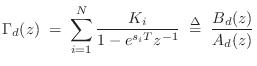
Since we have defined (in §7.2) the driving-point admittance $\Gamma (s)$ as the nominal transfer function of a system port, corresponding to defining the input as driving force and the output as resulting velocity (see Fig.7.3), we have that $\gamma(t)$ is defined as the system impulse response. Note, however, that the driving force and observed velocity need not be at the same physical point, and in general we may freely define any physical input and output points. Nevertheless, if the outputs are in velocity units and the inputs are in force units, then the transfer-function matrix will have units of admittance, and we will assume this for simplicity.

Sampling the impulse response can be expressed mathematically as $\gamma(t)\to T\gamma(nT) \to \gamma(n)$ .^9.2 In practice, we can only record a finite number of impulse-response samples. Usually a graceful taper (e.g., using the right half of an FFT window, such as the Hann window) yields better results than simple truncation. The system model is then implemented as a Finite Impulse Response (FIR) digital filter (§2.5.4). The next section describes the related impulse-invariant method for digital filter design which derives an infinite impulse response (IIR) digital filter that matches the analog filter impulse response exactly at the sampling times.

Sampling the impulse response has the advantage of preserving resonant frequencies (see next section), but its big disadvantage is aliasing of the frequency response. No ``system'' is truly bandlimited. For example, even a simple mass and dashpot with a nonzero initial condition produces a continuous decaying exponential response that is not bandlimited.

Before a continuous impulse response is sampled, a lowpass filter should be considered for eliminating all frequency components at half the sampling rate and above. In other words, the system itself should be ``lowpassed'' to avoid aliasing in many applications. (On the other hand, there are also many applications in which the frequency-response aliasing is not objectional to the ear.) If the system is linear and time invariant, and if we excite the system with input signals and initial conditions that are similarly bandlimited to less than half the sampling rate, no signal inside the system or appearing at the outputs will be aliased. In other words, these conditions yield an ideal bandlimited system simulation that remains exact (for the bandlimited signals) at the sampling instants.

Note, however, that time variation or nonlinearity (both common in practical instruments), together with feedback, will ``pump'' the signal spectrum higher and higher until aliasing is ultimately encountered (see §6.13). For this reason, feedback loops in the digital system may need additional lowpass filtering to attenuate newly generated high frequencies.

A sampled impulse response is an example of a nonparametric representation of a linear, time-invariant system. It is not usually regarded as a physical model, even when the impulse-response samples have a physical interpretation (such as when no anti-aliasing filter is used).

Impulse Invariant Method

The impulse-invariant method converts analog filter transfer functions to digital filter transfer functions in such a way that the impulse response is the same (invariant) at the sampling instants [343], [362, pp. 216-219]. Thus, if $\gamma(t)$ denotes the impulse-response of an analog (continuous-time) filter, then the digital (discrete-time) filter given by the impulse-invariant method will have impulse response $\gamma(nT)$ , where denotes the sampling interval in seconds. Moreover, the order of the filter is preserved, and IIR analog filters map to IIR digital filters. However, the digital filter's frequency response is an aliased version of the analog filter's frequency response.^9.3

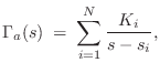
To derive the impulse-invariant method, we begin with the analog transfer function

$\displaystyle \Gamma_a(s) \isdefs \frac{B_a(s)}{A_a(s)} \isdefs \frac{b_a(0) s^... ...omment_mark>2028 s^{N} + a_a(1) s^{N-1} + \cdots + a_a(N-1)s + a_a(N)} \protect$

(9.1)

and perform a partial fraction expansion (PFE) down to first-order terms [449]:^9.4

$\displaystyle \Gamma_a(s) \eqsp \sum_{i=1}^N \frac{K_i}{s-s_i},$

where

is the

th pole of the analog system, and

is its residue [449]. Assume that the system is at least marginally stable [449] so that there are no poles in the right-half plane ( $\mbox{re\ensuremath{\left\{s_i\right\}}}\le 0$ ). Such a PFE is always possible when $\Gamma (s)$ is a strictly proper transfer function (more poles than zeros [449]).^9.5 Performing the inverse Laplace transform on the partial fraction expansion we obtain the impulse response in terms of the system poles and residues:

$\displaystyle \gamma_a(t) \eqsp \sum_{i=1}^N K_i e^{s_i t}, \quad t\ge 0.$

We now sample at intervals of

seconds to obtain the digital impulse response

$\displaystyle \gamma_d(n) \isdefs \gamma_a(nT) \eqsp \sum_{i=1}^N K_i e^{s_i nT}, \quad n= 0,1,2,\ldots\,.$

Taking the z transform gives the digital filter transfer function designed by the impulse-invariant method:

$\displaystyle \Gamma_d(z) \eqsp \sum_{i=1}^N \frac{K_i}{1 - e^{s_iT}z^{-1}} \isdefs \frac{B_d(z)}{A_d(z)}$

We see that the

-plane poles

have mapped to the

-plane poles

$\displaystyle \zbox {z_i \isdefs e^{s_iT}} \protect$

(9.2)

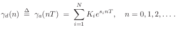
and the residues have remained unchanged. Clearly we must have $-\pi < \mbox{im\ensuremath{\left\{s_i\right\}}} T < \pi$ , i.e., the analog poles must lie within the bandwidth spanned by the digital sampling rate

. Otherwise, the pole angle $\mbox{im\ensuremath{\left\{s_i\right\}}} T$ will be aliased into the interval $[-\pi,\pi)$ . Stability is preserved since $\mbox{re\ensuremath{\left\{s_i\right\}}} \le 0 \;\Leftrightarrow\; \vert z_i\vert \le 1$ .

Note that the series combination of two digital filters designed by the impulse-invariant method is not impulse invariant. In other terms, the convolution of two sampled analog signals is not the same as the sampled convolution of those analog signals. This is easy to see when aliasing is considered. For example, let one signal be the impulse response of an ideal lowpass filter cutting off below half the sampling rate. Then this signal will not alias when sampled, and its convolution with any second signal will similarly not alias when sampled. However, if the second signal does alias upon sampling, then this aliasing is gone when the convolution precedes the sampling, and the results cannot be the same in the two cases.

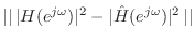
Matched Z Transformation

The matched z transformation uses the same pole-mapping Eq. $\,$ (8.2) as in the impulse-invariant method, but the zeros are handled differently. Instead of only mapping the poles of the partial fraction expansion and letting the zeros fall where they may, the matched z transformation maps both the poles and zeros in the factored form of the transfer function [362, pp. 224-226].

The factored form [449] of a transfer function

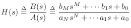
$\displaystyle H(s) \isdef \frac{B(s)}{A(s)} \isdef \frac{b_M s^M + \cdots b_1 s + b_0}{a_N s^N + \cdots a_1 s + a_0} \protect$

(9.3)

can be written as

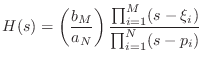
$\displaystyle H(s) = \left(\frac{b_M}{a_N}\right) \frac{\prod_{i=1}^M (s-\xi_i) }{\prod_{i=1}^N (s-p_i) } \protect$

(9.4)

The matched z transformation is carried out by replacing each first-order term of the form

by its digital equivalent $1 - e^{-aT}z^{-1}$ , i.e.,

$\displaystyle \zbox {s+a \;\to\; 1 - e^{-aT}z^{-1}} \protect$

(9.5)

to get

$\displaystyle H(s) = \left(\frac{b_M}{a_N}\right) \frac{ \prod_{i=1}^M (1 - e^{\xi_iT}z^{-1})}{ \prod_{i=1}^N (1 - e^{p_iT}z^{-1}} \protect$

(9.6)

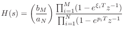
Thus, the matched z transformation normally yields different digital zeros than the impulse-invariant method. The impulse-invariant method is generally considered superior to the matched z transformation [343].

Relation to Finite Difference Approximation

The Finite Difference Approximation (FDA) (§7.3.1) is a special case of the matched transformation applied to the point . To see this, simply set in Eq. $\,$ (8.5) to obtain

$\displaystyle s \;\to\; 1 - z^{-1} \protect$

(9.7)

which is the FDA definition in the frequency domain given in Eq. $\,$ (7.3).

Since the FDA equals the match z transformation for the point , it maps analog dc () to digital dc () exactly. However, that is the only point on the frequency axis that is perfectly mapped, as shown in Fig.7.15.

Pole Mapping with Optimal Zeros

We saw in the preceding sections that both the impulse-invariant and the matched- transformations map poles from the left-half plane to the interior of the unit circle in the plane via

$\displaystyle z_i = e^{s_i T} \protect$

(9.8)

where

is the location of the

th pole in the

plane (assumed to lie in the strip $\vert\mbox{im\ensuremath{\left\{s\right\}}}\vert<\pi/T$ to avoid aliasing). The zeros, on the other hand, were different because the impulse-invariant method started with the partial fraction expansion while the matched-

transformation started with the factored form of the transfer function.

Therefore, an obvious generalization is to map the poles according to Eq. $\,$ (8.8), but compute the zeros in some optimal way, such as by Prony's method [449, p. 393],[273,297].

It is hard to do better Eq. $\,$ (8.8) as a pole mapping from to , when aliasing is avoided, because it preserves both the resonance frequency and bandwidth for a complex pole [449]. Therefore, good practical modeling results can be obtained by optimizing the zeros (residues) to achieve audio criteria given these fixed poles. Alternatively, only the least-damped poles need be constrained in this way, e.g., to fix and preserve the most important resonances of a stringed-instrument body or acoustic space.

Modal Expansion

A well known approach to transfer-function modeling is called modal synthesis, introduced in §1.3.9 [5,299,6,145,381,30]. Modal synthesis may be defined as constructing a source-filter synthesis model in which the filter transfer function is implemented as a sum of first- and/or second-order filter sections (i.e., as a parallel filter bank in which each filter is at most second-order--this was reviewed in §1.3.9). In other words, the physical system is represented as a superposition of individual modes driven by some external excitation (such as a pluck or strike).

In acoustics, the term mode of vibration, or normal mode, normally refers to a single-frequency spatial eigensolution of the governing wave equation. For example, the modes of an ideal vibrating string are the harmonically related sinusoidal string-shapes having an integer number of uniformly spaced zero-crossings (or nodes) along the string, including its endpoints. As first noted by Daniel Bernoulli (§A.2), acoustic vibration can be expressed as a superposition of component sinusoidal vibrations, i.e., as a superposition of modes.^9.6

When a single mode is excited by a sinusoidal driving force, all points of the physical object vibrate at the same temporal frequency (cycles per second), and the mode shape becomes proportional to the spatial amplitude envelope of the vibration. The sound emitted from the top plate of a guitar, for example, can be represented as a weighted sum of the radiation patterns of the respective modes of the top plate, where the weighting function is constructed according to how much each mode is excited (typically by the guitar bridge) [143,390,109,205,209].

The impulse-invariant method (§8.2), can be considered a special case of modal synthesis in which a continuous-time -plane transfer function is given as a starting point. More typically, modal synthesis starts with a measured frequency response, and a second-order parallel filter bank is fit to that in some way. In particular, any filter-design technique may be used (§8.6), followed by a conversion to second-order parallel form.

Modal expansions find extensive application in industry for determining parametric frequency responses (superpositions of second-order modes) from measured vibration data [299]. Each mode is typically parametrized in terms of its resonant frequency, bandwidth (or damping), and gain (most generally complex gain, to include phase).

Modal synthesis can also be seen as a special case of source-filter synthesis, which may be defined as any signal model based on factoring a sound-generating process into a filter driven by some (usually relatively simple) excitation signal. An early example of source-filter synthesis is the vocoder (§A.6.1). Whenever the filter in a source-filter model is implemented as a parallel second-order filter bank, we can call it modal synthesis (although, strictly speaking, each filter section should correspond to a resonant mode of the modeled resonant system).

Also related to modal synthesis is so-called formant synthesis, used extensively in speech synthesis [219,255,389,40,81,491,490,313,363,297]. A formant is simply a filter resonance having some center-frequency, bandwidth, and (sometimes specified) gain. Thus, a formant corresponds to a single mode of vibration in the vocal tract. Many text-to-speech systems in use today are based on the Klatt formant synthesizer for speech [255].

Since the importance of spectral formants in sound synthesis has more to do with the way we hear than with the physical parameters of a system, formant synthesis is probably best viewed as a spectral modeling synthesis method [456], as opposed to a physical modeling technique [435]. An exception to this rule may occur when the system consists physically of a parallel bank of second-order resonators, such as an array of tuning forks or Helmholtz resonators. In such a case, the mode parameters correspond to physically independent objects; this is of course rare in practice.

In the linear, time-invariant case, only modes in the range of human hearing need to be retained in the model. Also, any ``uncontrollable'' or ``unobservable'' modes should obviously be left out as well. With these simplificiation, the modal representation is generally more efficient than an explicit mass-spring-dashpot digitization (§7.3). On the other hand, since the modal representation is usually not directly physical, nonlinear extensions may be difficult and/or behave unnaturally.

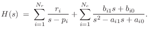
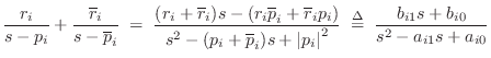
As in the impulse-invariant method (§8.2), starting with an order transfer function describing the input-output behavior of a physical system, a modal description can be obtained immediately from the partial fraction expansion (PFE):

$\displaystyle H(s) \isdefs \frac{B(s)}{A(s)} \isdefs \frac{b_M s^M + \cdots b_1... ..._0}{a_N s^N + \cdots a_1 s + a_0} \eqsp \sum_{i=1}^N \frac{r_i}{s-p_i} \protect$

(9.9)

where

denotes the

th pole, $\xi_i$ is the

th zero, and

is the residue of the

th pole [449]. (For simplicity of notation, Eq. $\,$ (8.9) is written for the case

and

distinct. See [449] for the details when this is not the case.) Since the system is real, complex poles will occur in complex conjugate pairs. This means that for each complex term

, the PFE will also include the complex-conjugate term $\overline{r}_i/(s-\overline{p}_i)$ . Such terms can be summed to create half as many real second-order terms:

$\displaystyle \frac{r_i}{s-p_i} + \frac{\overline{r}_i}{s-\overline{p}_i} \eqsp... ...vert p_i\right\vert^2} \isdefs \frac{b_{i1} s + b_{i0}}{s^2 - a_{i1}s + a_{i0}}$

(9.10)

Let

denote the number of complex pole pairs, and

be the number of real poles. Then the modal expansion can be written as

$\displaystyle H(s) \eqsp \sum_{i=1}^{N_r} \frac{r_i}{s-p_i} + \sum_{i=1}^{N_c} \frac{b_{i1} s + b_{i0}}{s^2 - a_{i1}s + a_{i0}}. \protect$

(9.11)

The real poles, if any, can be paired off into a sum of second-order sections as well, with one first-order section left over when

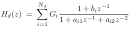
is odd. Note that each component second-order mode consists of one zero and two poles. The zero is necessary to adjust the phase of the resonant mode. The mode phase affects the frequency response at frequencies between resonances (from smoothly varying to the appearance of a deep notch somewhere between them).

A typical practical implementation of each mode in the sum is by means of second-order filter, or biquad section [449]. A biquad section is easily converted from continuous- to discrete-time form, such as by the impulse-invariant method of §8.2. The final discrete-time model then consist of a parallel bank of second-order digital filters

$\displaystyle H_d(z) \eqsp \sum_{i=1}^{N_d} G_i \frac{1 + b_i z^{-1}}{1 + a_{i1} z^{-1} + a_{i2} z^{-2}} \protect$

(9.12)

where

when the number of real poles is even, or

otherwise. The filter coefficients

and $a_{ij}$ are now digital second-order section coefficients which can be computed from the continuous-time filter coefficients, if they are known, or they can be directly estimated from discrete-time data.

Expressing complex poles of in polar form as $p_i \isdef R_i e^{j\theta_i}$ , (where now we assume denotes a pole in the plane), we obtain the classical relations [449]

$\displaystyle a_{i1}$	$\displaystyle =$	$\displaystyle p_i + \overline{p}_i \eqsp 2 R_i \cos(\theta_i) \protect$
$\displaystyle a_{i2}$	$\displaystyle =$	$\displaystyle \left\vert p_i\right\vert^2 \eqsp R_i^2. \protect$	(9.13)

These parameters are in turn related to the modal parameters resonance frequency

(Hz) and bandwidth

(Hz) by

$\begin{eqnarray*} \theta_i & = & 2\pi f_i / f_s\\ R_i & = & e^{-\pi B_i/f_s}. \end{eqnarray*}$

Often and are estimated from a measured log-magnitude frequency-response (see §8.8 for a discussion of various methods).

It remains to determine the overall section gain in Eq. $\,$ (8.12), and the coefficient determining the zero location. If (as is common in practice, since the human ear is not very sensitive to spectral nulls), then can be chosen to match the measured peak height. A particularly simple automatic method is to use least-squares minimization to compute using Eq. $\,$ (8.12) with $a_{i1}$ and $a_{i2}$ fixed (and ). Generally speaking, least-squares minimization is always immediate when the error to be minimized is linear in the unknown parameter (in this case ).

To estimate in Eq. $\,$ (8.12), an effective method is to work initially with a complex, first-order partial fraction expansion, and use least squares to determine complex gain coefficients for first-order (complex) terms of the form

$\displaystyle \frac{r_i}{s-p_i}$

as introduced in Eq. $\,$ (8.9) above. The angle and radius of

can still be determined by measuring peaks in the log-magnitude frequency response. When the first-order terms are paired and summed, the

coefficients will ``fall out.''

Sections implementing two real poles are not conveniently specified in terms of resonant frequency and bandwidth. In such cases, it is more common to work with the filter coefficients and directly, as they are often computed by system-identification software [288,428] or general purpose filter design utilities, such as in Matlab or Octave [443].

To summarize, numerous techniques exist for estimating modal parameters from measured frequency-response data, and some of these are discussed in §8.8 below. Specifically, resonant modes can be estimated from the magnitude, phase, width, and location of peaks in the Fourier transform of a recorded (or estimated) impulse response Another well known technique is Prony's method [449, p. 393], [297]. There is also a large literature on other methods for estimating the parameters of exponentially decaying sinusoids; examples include the matrix-pencil method [274], and parametric spectrum analysis in general [237].

State Space Approach to Modal Expansions

The preceding discussion of modal synthesis was based primarily on fitting a sum of biquads to measured frequency-response peaks. A more general way of arriving at a modal representation is to first form a state space model of the system [449], and then convert to the modal representation by diagonalizing the state-space model. This approach has the advantage of preserving system behavior between the given inputs and outputs. Specifically, the similarity transform used to diagonalize the system provides new input and output gain vectors which properly excite and observe the system modes precisely as in the original system. This procedure is especially more convenient than the transfer-function based approach above when there are multiple inputs and outputs. For some mathematical details, see [449]^9.7For a related worked example, see §C.17.6.

Delay Loop Expansion

When a subset of the resonating modes are nearly harmonically tuned, it can be much more computationally efficient to use a filtered delay loop (see §2.6.5) to generate an entire quasi-harmonic series of modes rather than using a biquad for each modal peak [439]. In this case, the resonator model becomes

$\displaystyle H(z) \eqsp \sum_{k=1}^N \frac{a_k}{1 - H_k(z) z^{-N_k}},$

where

is the length of the delay line in the

th comb filter, and

is a low-order filter which can be used to adjust finely the amplitudes and frequencies of the resonances of the

th comb filter [428]. Recall (Chapter 6) that a single filtered delay loop efficiently models a distributed 1D propagation medium such as a vibrating string or acoustic tube. More abstractly, a superposition of such quasi-harmonic mode series can provide a computationally efficient psychoacoustic equivalent approximation to arbitrary collections of modes in the range of human hearing.

Note that when is close to instead of , primarily only odd harmonic resonances are produced, as has been used in modeling the clarinet [431].

Frequency-Response Matching Using
Digital Filter Design Methods

Given force inputs and velocity outputs, the frequency response of an ideal mass was given in Eq. $\,$ (7.1.2) as

$\displaystyle \Gamma_m(j\omega) \eqsp \frac{1}{m j\omega},$

and the frequency response for a spring was given by Eq. $\,$ (7.1.3) as

$\displaystyle \Gamma_k(j\omega) \eqsp \frac{j\omega}{k}.$

Thus, an ideal mass is an integrator and an ideal spring is a differentiator. The modeling problem for masses and springs can thus be posed as a problem in digital filter design given the above desired frequency responses. More generally, the admittance frequency response ``seen'' at the port of a general

th-order LTI system is, from Eq. $\,$ (8.3),

$\displaystyle H(s) \isdefs \frac{B(s)}{A(s)} \isdefs \frac{b_M s^M + \cdots b_1 s + b_0}{a_N s^N + \cdots a_1 s + a_0} \protect$

(9.14)

where we assume

. Similarly, point-to-point ``trans-admittances'' can be defined as the velocity Laplace transform at one point on the physical object divided by the driving-force Laplace transform at some other point. There is also of course no requirement to always use driving force and observed velocity as the physical variables; velocity-to-force, force-to-force, velocity-to-velocity, force-to-acceleration, etc., can all be used to define transfer functions from one point to another in the system. For simplicity, however, we will prefer admittance transfer functions here.

Ideal Differentiator (Spring Admittance)

Figure 8.1 shows a graph of the frequency response of the ideal differentiator (spring admittance). In principle, a digital differentiator is a filter whose frequency response $H(e^{j\omega T})$ optimally approximates $j\omega$ for $\omega T$ between $-\pi$ and $\pi$ . Similarly, a digital integrator must match $1/j\omega$ along the unit circle in the plane. The reason an exact match is not possible is that the ideal frequency responses $j\omega$ and $1/j\omega$ , when wrapped along the unit circle in the plane, are not ``smooth'' functions any more (see Fig.8.1). As a result, there is no filter with a rational transfer function (i.e., finite order) that can match the desired frequency response exactly.

**Figure 8.1:** Imaginary part of the frequency response $H(e^{j\omega T})=j\omega$ of the ideal digital differentiator plotted over the unit circle in the plane (the real part being zero).
$\includegraphics[scale=0.9]{eps/f_ideal_diff_fr_cropped}$

The discontinuity at alone is enough to ensure that no finite-order digital transfer function exists with the desired frequency response. As with bandlimited interpolation (§4.4), it is good practice to reserve a ``guard band'' between the highest needed frequency $f_{\mbox{\tiny max}}$ (such as the limit of human hearing) and half the sampling rate . In the guard band $[f_{\mbox{\tiny max}},f_s/2]$ , digital filters are free to smoothly vary in whatever way gives the best performance across frequencies in the audible band $[0,f_{\mbox{\tiny max}}]$ at the lowest cost. Figure 8.2 shows an example. Note that, as with filters used for bandlimited interpolation, a small increment in oversampling factor yields a much larger decrease in filter cost (when the sampling rate is near $2f_{\mbox{\tiny max}}$ ).

In the general case of Eq. $\,$ (8.14) with $s=j\omega$ , digital filters can be designed to implement arbitrarily accurate admittance transfer functions by finding an optimal rational approximation to the complex function of a single real variable $\omega$

$\displaystyle H(e^{j\omega}) \eqsp \frac{B(j\omega)}{A(j\omega)} \eqsp \frac{b_... ...ega)^M + \cdots b_1 j\omega + b_0}{a_N (j\omega)^N + \cdots a_1 j\omega + a_0}$

over the interval $-\omega_{\mbox{\tiny max}}\leq \omega \leq \omega_{\mbox{\tiny max}}$ , where $\omega_{\mbox{\tiny max}}T<\pi$ is the upper limit of human hearing. For small guard bands $\delta\isdeftext \pi-\omega_{\mbox{\tiny max}}T$ , the filter order required for a given error tolerance is approximately inversely proportional to $\delta$ .

Digital Filter Design Overview

This section (adapted from [428]), summarizes some of the more commonly used methods for digital filter design aimed at matching a nonparametric frequency response, such as typically obtained from input/output measurements. This problem should be distinguished from more classical problems with their own specialized methods, such as designing lowpass, highpass, and bandpass filters [343,362], or peak/shelf equalizers [559,449], and other utility filters designed from a priori mathematical specifications.

The problem of fitting a digital filter to a prescribed frequency response may be formulated as follows. To simplify, we set .

Given a continuous complex function $H(e^{j\omega}),\,-\pi < \omega \le \pi$ , corresponding to a causal desired frequency response,^9.8 find a stable digital filter of the form

$\displaystyle {\hat H}(z) \isdefs \frac{{\hat B}(z)}{ {\hat A}(z)},$

where

$\displaystyle {\hat B}(z)$	$\displaystyle \isdef$	$\displaystyle {\hat b}_0 + {\hat b}_1 z^{-1} + \cdots + {\hat b}_{\hat{N}_b}z^{-{\hat{N}_b}}$	(9.15)
$\displaystyle {\hat A}(z)$	$\displaystyle \isdef$	$\displaystyle 1 + {\hat a}_1 z^{-1} + \cdots + {\hat a}_{\hat{N}_a}z^{-{\hat{N}_a}} ,$	(9.16)

with ${\hat{N}_b},{\hat{N}_a}$ given, such that some norm of the error

$\displaystyle J(\hat{\theta}) \isdefs \left\Vert\,H(e^{j\omega}) - {\hat H}(e^{j\omega})\,\right\Vert \protect$

(9.17)

is minimum with respect to the filter coefficients

$\displaystyle \hat{\theta}^K\isdefs [{\hat b}_0,{\hat b}_1,\ldots\,,{\hat b}_{\hat{N}_b},{\hat a}_1,{\hat a}_2,\ldots\,,{\hat a}_{\hat{N}_a}].$

The filter coefficients are constrained to lie in some subset $\hat{\Theta}\subset\Re ^{{\hat N}}$ , where ${\hat N}\isdef {\hat{N}_a}+{\hat{N}_b}+1$ . The filter coefficients may also be complex, in which case $\hat{\Theta}\subset{\bf C}^{{\hat N}}$ .

The approximate filter ${\hat H}$ is typically constrained to be stable, and since ${\hat B}(z)$ is causal (no positive powers of ), stability implies causality. Consequently, the impulse response of the model ${\hat h}(n)$ is zero for .

The filter-design problem is then to find a (strictly) stable ${\hat{N}_a}$ -pole, ${\hat{N}_b}$ -zero digital filter which minimizes some norm of the error in the frequency-response. This is fundamentally rational approximation of a complex function of a real (frequency) variable, with constraints on the poles.

While the filter-design problem has been formulated quite naturally, it is difficult to solve in practice. The strict stability assumption yields a compact space of filter coefficients $\hat{\Theta}$ , leading to the conclusion that a best approximation $\hat{H}^\ast$ exists over this domain.^9.9Unfortunately, the norm of the error $J(\hat{\theta})$ typically is not a convex^9.10function of the filter coefficients on $\hat{\Theta}$ . This means that algorithms based on gradient descent may fail to find an optimum filter due to their premature termination at a suboptimal local minimum of $J(\hat{\theta})$ .

Fortunately, there is at least one norm whose global minimization may be accomplished in a straightforward fashion without need for initial guesses or ad hoc modifications of the complex (phase-sensitive) IIR filter-design problem--the Hankel norm [155,428,177,36]. Hankel norm methods for digital filter design deliver a spontaneously stable filter of any desired order without imposing coefficient constraints in the algorithm.

An alternative to Hankel-norm approximation is to reformulate the problem, replacing Eq. $\,$ (8.17) with a modified error criterion so that the resulting problem can be solved by linear least-squares or convex optimization techniques. Examples include

Pseudo-norm minimization: (Pseudo-norms can be zero for nonzero functions.) For example, Padé approximation falls in this category. In Padé approximation, the first ${\hat{N}_a}+{\hat{N}_b}+1$ samples of the impulse-response of are matched exactly, and the error in the remaining impulse-response samples is ignored.
Ratio Error: Minimize $\vert\vert\,H(e^{j\omega})/{\hat H}(e^{j\omega})\,\vert\vert$ subject to ${\hat B}(z)=1$ . Minimizing the norm of the ratio error yields the class of methods known as linear prediction techniques [20,296,297]. Since, by the definition of a norm, we have $\vert\vert\,e^{j\theta}E(e^{j\omega})\,\vert\vert = \vert\vert\,E(e^{j\omega})\,\vert\vert$ , it follows that $\vert\vert\,H/{\hat H}\,\vert\vert = \vert\vert\,\vert H\vert/\vert{\hat H}\vert\,\vert\vert$ ; therefore, ratio error methods ignore the phase of the approximation. It is also evident that ratio error is minimized by making $\vert{\hat H}(e^{j\omega})\vert$ larger than $\vert H(e^{j\omega})\vert$ .^9.11 For this reason, ratio-error methods are considered most appropriate for modeling the spectral envelope of $\vert H(e^{j\omega})\vert$ . It is well known that these methods are fast and exceedingly robust in practice, and this explains in part why they are used almost exclusively in some data-intensive applications such as speech modeling and other spectral-envelope applications. In some applications, such as adaptive control or forecasting, the fact that linear prediction error is minimized can justify their choice.
Equation error: Minimize

$\displaystyle \left\Vert\,{\hat A}(e^{j\omega})H(e^{j\omega})-{\hat B}(e^{j\ome... ...}(e^{j\omega})\left[ H(e^{j\omega})-{\hat H}(e^{j\omega})\right]\,\right\Vert.$
When the norm of equation-error is minimized, the problem becomes solving a set of ${\hat N}={\hat{N}_a}+{\hat{N}_b}+1$ linear equations.
The above expression makes it clear that equation-error can be seen as a frequency-response error weighted by $\vert{\hat A}(e^{j\omega})\vert$ . Thus, relatively large errors can be expected where the poles of the optimum approximation (roots of ${\hat A}(z)$ ) approach the unit circle $\vert z\vert=1$ . While this may make the frequency-domain formulation seem ill-posed, in the time-domain, linear prediction error is minimized in the sense, and in certain applications this is ideal. (Equation-error methods thus provide a natural extension of ratio-error methods to include zeros.) Using so-called Steiglitz-McBride iterations [287,449,288], the equation-error solution iteratively approaches the norm-minimizing solution of Eq. $\,$ (8.17) for the L2 norm.
Examples of minimizing equation error using the matlab function invfreqz are given in §8.6.3 and §8.6.4 below. See [449, Appendix I] (based on [428, pp. 48-50]) for a discussion of equation-error IIR filter design and a derivation of a fast equation-error method based on the Fast Fourier Transform (FFT) (used in invfreqz).
Conversion to real-valued approximation: For example, power spectrum matching, i.e., minimization of $\vert\vert\,\vert H(e^{j\omega})\vert^2-\vert{\hat H}(e^{j\omega})\vert^2\,\vert\vert$ , is possible using the Chebyshev or norm [428]. Similarly, linear-phase filter design can be carried out with some guarantees, since again the problem reduces to real-valued approximation on the unit circle. The essence of these methods is that the phase-response is eliminated from the error measure, as in the norm of the ratio error, in order to convert a complex approximation problem into a real one. Real rational approximation of a continuous curve appears to be solved in principle only under the norm [373,374].
Decoupling poles and zeros: An effective example of this approach is Kopec's method [428] which consists of using ratio error to find the poles, computing the error spectrum $E=H/{\hat H}$ , inverting it, and fitting poles again (to $1/E(e^{j\omega})$ ). There is a wide variety of methods which first fit poles and then zeros. None of these methods produce optimum filters, however, in any normal sense.

In addition to these modifications, sometimes it is necessary to reformulate the problem in order to achieve a different goal. For example, in some audio applications, it is desirable to minimize the log-magnitude frequency-response error. This is due to the way we hear spectral distortions in many circumstances. A technique which accomplishes this objective to the first order in the norm is described in [428].

Sometimes the most important spectral structure is confined to an interval of the frequency domain. A question arises as to how this structure can be accurately modeled while obtaining a cruder fit elsewhere. The usual technique is a weighting function versus frequency. An alternative, however, is to frequency-warp the problem using a first-order conformal map. It turns out a first-order conformal map can be made to approximate very well frequency-resolution scales of human hearing such as the Bark scale or ERB scale [459]. Frequency-warping is especially valuable for providing an effective weighting function connection for filter-design methods, such as the Hankel-norm method, that are intrinsically do not offer choice of a weighted norm for the frequency-response error.

There are several methods which produce ${\hat H}(z){\hat H}(z^{-1})$ instead of ${\hat H}(z)$ directly. A fast spectral factorization technique is useful in conjunction with methods of this category [428]. Roughly speaking, a size $2{\hat{N}_a}$ polynomial factorization is replaced by an FFT and a size ${\hat{N}_a}$ system of linear equations.

Digital Differentiator Design

We saw the ideal digital differentiator frequency response in Fig.8.1, where it was noted that the discontinuity in the response at $\omega=\pm\pi$ made an ideal design unrealizable (infinite order). Fortunately, such a design is not even needed in practice, since there is invariably a guard band between the highest supported frequency $f_{\mbox{\tiny max}}$ and half the sampling rate .

**Figure 8.2:** FIR differentiator designed by the matlab function `invfreqz` (Octave). Top: Overlay of the ideal amplitude response ( $\vert j2\pi f\vert$ ), fitted filter amplitude response, and guard-band limit (at 20 kHz). Bottom: Overlay of ideal phase response ( $\pi /2$ radians), fitted filter phase response, and guard-band limit (20 kHz).
$\includegraphics[width=\twidth]{eps/iirdiff-mag-phs-N0-M10}$

Figure 8.2 illustrates a more practical design specification for the digital differentiator as well as the performance of a tenth-order FIR fit using invfreqz (which minimizes equation error) in Octave.^9.12 The weight function passed to invfreqz was 1 from 0 to 20 kHz, and zero from 20 kHz to half the sampling rate (24 kHz). Notice how, as a result, the amplitude response follows that of the ideal differentiator until 20 kHz, after which it rolls down to a gain of 0 at 24 kHz, as it must (see Fig.8.1). Higher order fits yield better results. Using poles can further improve the results, but the filter should be checked for stability since invfreqz designs filters in the frequency domain and does not enforce stability.^9.13

Fitting Filters to Measured Amplitude Responses

The preceding filter-design example digitized an ideal differentiator, which is an example of converting an LTI lumped modeling element into a digital filter while maximally preserving its frequency response over the audio band. Another situation that commonly arises is the need for a digital filter that matches a measured frequency response over the audio band.

Measured Amplitude Response

Figure 8.3 shows a plot of simulated amplitude-response measurements at 10 frequencies equally spread out between 100 Hz and 3 kHz on a log frequency scale. The ``measurements'' are indicated by circles. Each circle plots, for example, the output amplitude divided by the input amplitude for a sinusoidal input signal at that frequency [449]. These ten data points are then extended to dc and half the sampling rate, interpolated, and resampled to a uniform frequency grid (solid line in Fig.8.3), as needed for FFT processing. The details of these computations are listed in Fig.8.4. We will fit a four-pole, one-zero, digital-filter frequency-response to these data.^9.14

**Figure 8.3:** Example measured amplitude-response samples at 10 exponentially spaced frequencies. Circles: Measured amplitude-response points. Solid: Extrapolated, spline-interpolated, and uniformly resampled amplitude response, ready for `ifft`.
$\includegraphics[width=\twidth]{eps/tmps2-G}$

**Figure:** Script (matlab) for simulating a measured amplitude response at 10 exponentially spaced frequencies and extrapolating/interpolating/resampling to obtain a complete, nonparametric amplitude response, uniformly sampled at FFT frequencies. This script generated Fig.8.3.
NZ = 1; % number of ZEROS in the filter to be designed NP = 4; % number of POLES in the filter to be designed NG = 10; % number of gain measurements fmin = 100; % lowest measurement frequency (Hz) fmax = 3000; % highest measurement frequency (Hz) fs = 10000; % discrete-time sampling rate Nfft = 512; % FFT size to use df = (fmax/fmin)^(1/(NG-1)); % uniform log-freq spacing f = fmin * df .^ (0:NG-1); % measurement frequency axis % Gain measurements (synthetic example = triangular amp response): Gdb = 10[1:NG/2,NG/2:-1:1]/(NG/2); % between 0 and 10 dB gain % Must decide on a dc value. % Either use what is known to be true or pick something "maximally % smooth". Here we do a simple linear extrapolation: dc_amp = Gdb(1) - f(1)(Gdb(2)-Gdb(1))/(f(2)-f(1)); % Must also decide on a value at half the sampling rate. % Use either a realistic estimate or something "maximally smooth". % Here we do a simple linear extrapolation. While zeroing it % is appealing, we do not want any zeros on the unit circle here. Gdb_last_slope = (Gdb(NG) - Gdb(NG-1)) / (f(NG) - f(NG-1)); nyq_amp = Gdb(NG) + Gdb_last_slope * (fs/2 - f(NG)); Gdbe = [dc_amp, Gdb, nyq_amp]; fe = [0,f,fs/2]; NGe = NG+2; % Resample to a uniform frequency grid, as required by ifft. % We do this by fitting cubic splines evaluated on the fft grid: Gdbei = spline(fe,Gdbe); % say `help spline' fk = fs[0:Nfft/2]/Nfft; % fft frequency grid (nonneg freqs) Gdbfk = ppval(Gdbei,fk); % Uniformly resampled amp-resp figure(1); semilogx(fk(2:end-1),Gdbfk(2:end-1),'-k'); grid('on'); axis([fmin/2 fmax2 -3 11]); hold('on'); semilogx(f,Gdb,'ok'); xlabel('Frequency (Hz)'); ylabel('Magnitude (dB)'); title(['Measured and Extrapolated/Interpolated/Resampled ',... 'Amplitude Response']);

Figure: Script (matlab) for simulating a measured amplitude response at 10 exponentially spaced frequencies and extrapolating/interpolating/resampling to obtain a complete, nonparametric amplitude response, uniformly sampled at FFT frequencies. This script generated Fig.8.3.

NZ = 1;      % number of ZEROS in the filter to be designed
NP = 4;      % number of POLES in the filter to be designed
NG = 10;     % number of gain measurements
fmin = 100;  % lowest measurement frequency (Hz)
fmax = 3000; % highest measurement frequency (Hz)
fs = 10000;  % discrete-time sampling rate
Nfft = 512;  % FFT size to use
df = (fmax/fmin)^(1/(NG-1)); % uniform log-freq spacing
f = fmin * df .^ (0:NG-1);   % measurement frequency axis

% Gain measurements (synthetic example = triangular amp response):
Gdb = 10*[1:NG/2,NG/2:-1:1]/(NG/2); % between 0 and 10 dB gain

% Must decide on a dc value.
% Either use what is known to be true or pick something "maximally
% smooth".  Here we do a simple linear extrapolation:
dc_amp = Gdb(1) - f(1)*(Gdb(2)-Gdb(1))/(f(2)-f(1));

% Must also decide on a value at half the sampling rate.
% Use either a realistic estimate or something "maximally smooth".
% Here we do a simple linear extrapolation. While zeroing it
% is appealing, we do not want any zeros on the unit circle here.
Gdb_last_slope = (Gdb(NG) - Gdb(NG-1)) / (f(NG) - f(NG-1));
nyq_amp = Gdb(NG) + Gdb_last_slope * (fs/2 - f(NG));

Gdbe = [dc_amp, Gdb, nyq_amp];
fe = [0,f,fs/2];
NGe = NG+2;

% Resample to a uniform frequency grid, as required by ifft.
% We do this by fitting cubic splines evaluated on the fft grid:
Gdbei = spline(fe,Gdbe); % say `help spline'
fk = fs*[0:Nfft/2]/Nfft; % fft frequency grid (nonneg freqs)
Gdbfk = ppval(Gdbei,fk); % Uniformly resampled amp-resp

figure(1);
semilogx(fk(2:end-1),Gdbfk(2:end-1),'-k'); grid('on');
axis([fmin/2 fmax*2 -3 11]);
hold('on'); semilogx(f,Gdb,'ok');
xlabel('Frequency (Hz)');   ylabel('Magnitude (dB)');
title(['Measured and Extrapolated/Interpolated/Resampled ',...
       'Amplitude Response']);

Desired Impulse Response

It is good to check that the desired impulse response is not overly aliased in the time domain. The impulse-response for this example is plotted in Fig.8.5. We see that it appears quite short compared with the inverse FFT used to compute it. The script in Fig.8.6 gives the details of this computation, and also prints out a measure of ``time-limitedness'' defined as the norm of the outermost 20% of the impulse response divided by its total norm--this measure was reported to be % for this example.

**Figure:** Desired impulse response obtained from a length 512 inverse FFT of the interpolated measured amplitude response in Fig.8.3.
$\includegraphics[width=\twidth]{eps/tmps2-ir}$

Note also that the desired impulse response is noncausal. In fact, it is zero phase [449]. This is of course expected because the desired frequency response was real (and nonnegative).

**Figure 8.6:** Script (matlab) for checking the desired impulse-response for time aliasing. If it wraps around in the time buffer, one can increase the inverse FFT length (`Nfft`) and/or smooth the desired amplitude response (`Sdb`).
Ns = length(Gdbfk); if Ns~=Nfft/2+1, error("confusion"); end Sdb = [Gdbfk,Gdbfk(Ns-1:-1:2)]; % install negative-frequencies S = 10 .^ (Sdb/20); % convert to linear magnitude s = ifft(S); % desired impulse response s = real(s); % any imaginary part is quantization noise tlerr = 100norm(s(round(0.9Ns:1.1*Ns)))/norm(s); disp(sprintf(['Time-limitedness check: Outer 20%% of impulse ' ... 'response is %0.2f %% of total rms'],tlerr)); % = 0.02 percent if tlerr>1.0 % arbitrarily set 1% as the upper limit allowed error('Increase Nfft and/or smooth Sdb'); end figure(2); plot(s,'-k'); grid('on'); title('Impulse Response'); xlabel('Time (samples)'); ylabel('Amplitude');

Ns = length(Gdbfk); if Ns~=Nfft/2+1, error("confusion"); end
Sdb = [Gdbfk,Gdbfk(Ns-1:-1:2)]; % install negative-frequencies

S = 10 .^ (Sdb/20); % convert to linear magnitude
s = ifft(S); % desired impulse response
s = real(s); % any imaginary part is quantization noise
tlerr = 100*norm(s(round(0.9*Ns:1.1*Ns)))/norm(s);
disp(sprintf(['Time-limitedness check: Outer 20%% of impulse ' ...
              'response is %0.2f %% of total rms'],tlerr));
% = 0.02 percent
if tlerr>1.0 % arbitrarily set 1% as the upper limit allowed
  error('Increase Nfft and/or smooth Sdb');
end

figure(2);
plot(s,'-k'); grid('on');   title('Impulse Response');
xlabel('Time (samples)');   ylabel('Amplitude');

Converting the Desired Amplitude Response to Minimum Phase

Phase-sensitive filter-design methods such as the equation-error method implemented in invfreqz are normally constrained to produce filters with causal impulse responses.^9.15 In cases such as this (phase-sensitive filter design when we don't care about phase--or don't have it), it is best to compute the minimum phase corresponding to the desired amplitude response [449].

As detailed in Fig.8.8, the minimum phase is constructed by the cepstral method [449].^9.16

The four-pole, one-zero filter fit using invfreqz is shown in Fig.8.7.

**Figure 8.7:** Overlay of desired amplitude response (solid) and that of a fourth-order filter fit (dashed) using `invfreqz`.
$\includegraphics[width=\twidth]{eps/tmps2-Hh}$

**Figure:** Script (matlab) for converting the (real) desired amplitude response to minimum-phase form for `invfreqz`. This script generated Fig.8.7.
c = ifft(Sdb); % compute real cepstrum from log magnitude spectrum % Check aliasing of cepstrum (in theory there is always some): caliaserr = 100norm(c(round(Ns0.9:Ns1.1)))/norm(c); disp(sprintf(['Cepstral time-aliasing check: Outer 20%% of ' ... 'cepstrum holds %0.2f %% of total rms'],caliaserr)); % = 0.09 percent if caliaserr>1.0 % arbitrary limit error('Increase Nfft and/or smooth Sdb to shorten cepstrum'); end % Fold cepstrum to reflect non-min-phase zeros inside unit circle: % If complex: % cf=[c(1),c(2:Ns-1)+conj(c(Nfft:-1:Ns+1)),c(Ns),zeros(1,Nfft-Ns)]; cf = [c(1), c(2:Ns-1)+c(Nfft:-1:Ns+1), c(Ns), zeros(1,Nfft-Ns)]; Cf = fft(cf); % = dB_magnitude + j minimum_phase Smp = 10 .^ (Cf/20); % minimum-phase spectrum Smpp = Smp(1:Ns); % nonnegative-frequency portion wt = 1 ./ (fk+1); % typical weight fn for audio wk = 2pifk/fs; [B,A] = invfreqz(Smpp,wk,NZ,NP,wt); Hh = freqz(B,A,Ns); figure(3); plot(fk,db([Smpp(:),Hh(:)])); grid('on'); xlabel('Frequency (Hz)'); ylabel('Magnitude (dB)'); title('Magnitude Frequency Response'); % legend('Desired','Filter');

c = ifft(Sdb); % compute real cepstrum from log magnitude spectrum
% Check aliasing of cepstrum (in theory there is always some):
caliaserr = 100*norm(c(round(Ns*0.9:Ns*1.1)))/norm(c);
disp(sprintf(['Cepstral time-aliasing check: Outer 20%% of ' ...
    'cepstrum holds %0.2f %% of total rms'],caliaserr));
% = 0.09 percent
if caliaserr>1.0 % arbitrary limit
  error('Increase Nfft and/or smooth Sdb to shorten cepstrum');
end
% Fold cepstrum to reflect non-min-phase zeros inside unit circle:
% If complex:
% cf=[c(1),c(2:Ns-1)+conj(c(Nfft:-1:Ns+1)),c(Ns),zeros(1,Nfft-Ns)];
cf = [c(1), c(2:Ns-1)+c(Nfft:-1:Ns+1), c(Ns), zeros(1,Nfft-Ns)];
Cf = fft(cf); % = dB_magnitude + j * minimum_phase
Smp = 10 .^ (Cf/20); % minimum-phase spectrum

Smpp = Smp(1:Ns); % nonnegative-frequency portion
wt = 1 ./ (fk+1); % typical weight fn for audio
wk = 2*pi*fk/fs;
[B,A] = invfreqz(Smpp,wk,NZ,NP,wt);
Hh = freqz(B,A,Ns);

figure(3);
plot(fk,db([Smpp(:),Hh(:)])); grid('on');
xlabel('Frequency (Hz)');
ylabel('Magnitude (dB)');
title('Magnitude Frequency Response');
% legend('Desired','Filter');

Commuted Synthesis

In acoustic stringed musical instruments such as guitars and pianos, the strings couple via a ``bridge'' to some resonating acoustic structure (typically made of wood) that is required for efficient transduction of string vibration to acoustic propagation in the surrounding air. The resonator also imposes its own characteristic frequency response on the radiated sound. Spectral characteristics of the string excitation, the string resonances, and body/soundboard/enclosure resonator, are thus combined multiplicatively in the radiated sound, as depicted in Fig. 8.9.

**Figure 8.9:** Schematic diagram of a stringed musical instrument.
$\includegraphics[width=\twidth]{eps/guitar}$

The idea of commuted synthesis is that, because the string and body are close to linear and time-invariant, we may commute the string and resonator, as shown in Fig. 8.10.

**Figure 8.10:** Equivalent diagram in the linear, time-invariant case.
$\includegraphics[width=\twidth]{eps/commuted_guitar}$

The excitation can now be convolved with the resonator impulse response to provide a single, aggregate, excitation table, as depicted in Fig. 8.11. This is the basic idea behind commuted synthesis, and it greatly reduces the complexity of stringed instrument implementations, since the body filter is replaced by an inexpensive lookup table [439,230]. These simplifications are presently important in single-processor polyphonic synthesizers such as multimedia DSP chips.

**Figure 8.11:** Use of an aggregate excitation given by the convolution of original excitation with the resonator impulse response.
$\includegraphics[scale=0.9]{eps/fexcitation}$

In the simplest case, the string is ``plucked'' using the (half-windowed) impulse response of the body.

An example of an excitation is the force applied by a pick or a finger at some point, or set of points, along the string. The input force per sample at each point divided by gives the velocity to inject additively at that point in both traveling-wave directions. (The factor of comes from splitting the injected velocity into two traveling-wave components, and from the fact that two string end-points are being driven.) Equal injection in the left- and right-going directions corresponds to an excitation force which is stationary with respect to the string.

**Figure 8.12:** Possible components of a guitar resonator.
$\includegraphics[width=\twidth]{eps/guitar_resonator_components}$

In a practical instrument, the ``resonator'' is determined by the choice of output signal in the physical scenario, and it generally includes filtering downstream of the body itself, as shown in Fig. 8.12. A typical example for the guitar or violin would be to choose the output signal at a point a few feet away from the top plate of the body. In practice, such a signal can be measured using a microphone held at the desired output point and recording the response at that point to the striking of the bridge with a force hammer. It is useful to record simultaneously the output of an accelerometer mounted on the bridge in order to also obtain experimentally the driving-point impedance at the bridge. In general, it is desirable to choose the output close to the instrument so as to keep the resonator response as short as possible. The resonator components need to be linear and time invariant, so they will be commutative with the string and combinable with the string excitation signal via convolution.

The string should also be linear and time invariant in order to be able to commute it with the generalized resonator. However, the string is actually the least linear element of most stringed musical instruments, with the main effect of nonlinearity being often a slight increase of the fundamental vibration frequency with amplitude. A secondary effect is to introduce coupling between the two polarizations of vibration along the length of the string. In practice, however, the string can be considered sufficiently close to linear to permit commuting with the body. The string is also time varying in the presence of vibrato, but this too can be neglected in practice. While commuting a live string and resonator may not be identical mathematically, the sound is substantially the same.

There are various options when combining the excitation and resonator into an aggregate excitation, as shown in Fig. 8.11. For example, a wave-table can be prepared which contains the convolution of a particular point excitation with a particular choice of resonator. Perhaps the simplest choice of excitation is the impulse signal. Physically, this would be natural when the wave variables in the string are taken to be acceleration waves for a plucked string; in this case, an ideal pluck gives rise to an impulse of acceleration input to the left and right in the string at the pluck point. If loss of perceived pick position is unimportant, the impulse injection need only be in a single direction. (The comb filtering which gives rise to the pick-position illusion can be restored by injecting a second, negated impulse at a delay equal to the travel time to and from the bridge.) In this simple case of a single impulse to pluck the string, the aggregate excitation is simply the impulse response of the resonator. Many excitation and resonator variations can be simulated using a collection of aggregate excitation tables. It is useful to provide for interpolation of excitation tables so as to provide intermediate points along a parameter dimension. In fact, all the issues normally associated with sampling synthesis arise in the context of the string excitation table. A disadvantage of combining excitation and resonator is the loss of multiple output signals from the body simulation, but the timbral effects arising from the mixing together of multiple body outputs can be obtained via a mixing of corresponding excitation tables.

If the aggregate excitation is too long, it may be shortened by a variety of techniques. It is good to first convert the signal to minimum phase so as to provide the maximum shortening consistent with the original magnitude spectrum. Secondly, can be windowed using the right wing of any window function typically used in spectrum analysis. An interesting choice is the exponential window, since it has the interpretation of increasing the resonator damping in a uniform manner, i.e., all the poles and zeros of the resonator are contracted radially in the plane by the same factor.

Body-Model Factoring

In commuted synthesis, it is often helpful to factor out the least-damped resonances in the body model for implementation in parametric form (e.g., as second-order filters, or ``biquads''). The advantages of this are manifold, including the following:

The excitation table is shortened (now containing only the most damped modal components).
The excitation table signal-to-quantization-noise ratio is improved.
The most important resonances remain parametric, facilitating real-time control. In other words, the parametric resonances can be independently modulated to produce interesting effects.
Multiple body outputs become available from the parametric filters.
Resonators may be already available in a separate effects unit, making them ``free.''
A memory vs. computation trade-off is available for cost optimization.

Techniques for carrying out this factorization in practice are discussed in §8.8 [229].

Extracting Parametric Resonators from a Nonparametric Impulse Response

As mentioned in §8.7.1 above, a valuable way of shortening the excitation table in commuted synthesis is to factor the body resonator into its most-damped and least-damped modes. The most-damped modes are then commuted and combined with the excitation in impulse-response form. The least-damped modes can be left in parametric form as recursive digital filter sections.

Commuted synthesis is a technique in which the body resonator is commuted with the string model, as shown in Fig.8.10, in order to avoid having to implement a large body filter at all [439,232,229].^9.18In commuted synthesis, the excitation (e.g., plucking force versus time) can be convolved with the resonator impulse response to provide a single aggregate excitation signal. This signal is short enough to store in a look-up table, and a note is played by simply summing it into the string.

Mode Extraction Techniques

The goal of resonator factoring is to identify and remove the least-damped resonant modes of the impulse response. In principle, this means ascertaining the precise resonance frequencies and bandwidths associated with each of the narrowest ``peaks'' in the resonator frequency response, and dividing them out via inverse filtering, so they can be implemented separately as resonators in series. If in addition the amplitude and phase of a resonance peak are accurately measurable in the complex frequency response, the mode can be removed by complex spectral subtraction (equivalent to subtracting the impulse-response of the resonant mode from the total impulse response); in this case, the parametric modes are implemented in a parallel bank as in [66]. However, in the parallel case, the residual impulse response is not readily commuted with the string.

In the inverse-filtering case, the factored resonator components are in cascade (series) so that the damped modes left behind may be commuted with the string and incorporated in the excitation table by convolving the residual impulse response with the desired string excitation signal. In the parallel case, the damped modes do not commute with the string since doing so would require somehow canceling them in the parallel filter sections. In principle, the string would have to be duplicated so that one instance can be driven by the residual signal with no body resonances at all, while the other is connected to the parallel resonator bank and driven only by the natural string excitation without any commuting of string and resonator. Since duplicating the string is unlikely to be cost-effective, the impulse response of the high-frequency modes can be commuted and convolved with the string excitation as in the series case to obtain qualitative results. The error in doing this is that the high-frequency modes are being multiplied by the parallel resonators rather than being added to them.

Various methods are available for estimating the mode parameters for inverse filtering:

Amplitude response peak measurement
Weighted digital filter design
Linear prediction
Sinusoidal modeling
Late impulse-response analysis

Amplitude response peak measurement

The longest ringing modes are associated with the narrowest bandwidths. When they are important resonances in the frequency response, they also tend to be the tallest peaks in the frequency response magnitude. (If they are not the tallest near the beginning of the impulse response, they will be the tallest near the end.) Therefore, one effective technique for measuring the least-damped resonances is simply to find the precise location and width of the narrowest and tallest spectral peaks in the measured amplitude response of the resonator. The center-frequency and bandwidth of a narrow frequency-response peak determine two poles in the resonator to be factored out. Expressing a filter in terms of its poles and zeros is one type of ``parametric'' filter representation, as opposed to ``nonparametric'' representations such as the impulse response or frequency response. Prony's method [449,297,273] is one well known technique for estimating the frequencies and bandwidths of sums of exponentially decaying sinusoids (two-pole resonator impulse responses).

In the factoring example presented in §8.8.6, the frequency and bandwidth of the main Helmholtz air mode are measured manually using an interactive spectrum analysis tool. However, it is a simple matter to automate peak-finding in FFT magnitude data. (See, for example, the peak finders used in sinusoidal modeling, discussed a bit further in §8.8.1 below.)

Weighted digital filter design

**Figure 8.13:** Illustration of one way to determine the parameters of a least-damped resonant mode.
$\includegraphics[width=0.8\twidth]{eps/fbrUsingInvfreqz}$

Many methods for digital filter design support spectral weighting functions that can be used to focus in on the least-damped modes in the frequency response. One is the weighted equation-error method which is available in the matlab invfreqz() function (§8.6.4). Figure 8.13 illustrates use of it. For simplicity, only one frequency-response peak plus noise is shown in this synthetic example. First, the peak center-frequency is measured using a quadratically interpolating peak finder operating on the dB spectral magnitude. This is used to set the spectral weighting function. Next, invfreqz() is called to design a two-pole filter having a frequency response that approximates the measured data as closely as possible. The weighting function is also shown in Fig.8.13, renormalized to overlay on the scale of the plot. Finally, the amplitude response of the two-pole filter designed by the equation-error method is shown overlaid in the figure. Note that the agreement is quite good near the peak which is what matters most. The interpolated peak frequency measured initially in the nonparametric spectral magnitude data can be used to fine-tune the pole-angles of the designed filter, thus rendering the equation-error method a technique for measuring only the peak bandwidth in this case. There are of course many, many techniques in the signal processing literature for measuring spectral peaks.

Linear prediction

Another well known method for converting the least-damped modes into parametric form is Linear Predictive Coding (LP) followed by polynomial factorization to obtain resonator poles. LP is particularly good at fitting spectral peaks due to the nature of the error criterion it minimizes [428]. The poles closest to the unit circle in the plane can be chosen for the ``ringy'' part of the resonator. It is well known that when using techniques like LP to model spectral peaks for extraction, orders substantially higher than twice the number of spectral peaks should be used. The extra degrees of freedom in the LP fit give more poles for modeling spectral detail other than the peaks, allowing the poles modeling the peaks to fit them with less distraction. On the other hand, if the order chosen is too high, sometimes more than two poles will home in on the same peak. In some cases, this may be appropriate since the body resonances are not necessary resolvable so as to separate the peaks, especially at high frequencies.

Sinusoidal modeling

Another way to find the least-damped mode parameters is by means of an intermediate sinusoidal model of the body impulse response, or, more appropriately, the energy decay relief (EDR) computed from the body impulse response (see §3.2.2). Such sinusoidal models have been used to determine the string loop filter in digital waveguide strings models. In the case of string loop-filter estimation, the sinusoidal model is applied to the impulse response (or ``pluck'' response) of a vibrating string or acoustic tube. In the present application, it is ideally applied to the EDR of the body impulse response (or ``hammer-strike'' response).

Since sinusoidal modeling software (e.g. [424]) typically quadratically interpolates the peak frequencies, the resonance frequencies are generally quite accurately estimated provided the frame size is chosen large enough to span many cycles of the underlying resonance.

The sinusoidal amplitude envelopes yield a particularly robust measurement of resonance bandwidth. Theoretically, the modal decay should be exponential. Therefore, on a dB scale, the amplitude envelope should decay linearly. Linear regression can be used to fit a straight line to the measured log-amplitude envelope of the impulse response of each long-ringing mode. Note that even when amplitude modulation is present due to modal couplings, the ripples tend to average out in the regression and have little effect on the slope measurement. This robustness can be enhanced by starting and ending the linear regression on local maxima in the amplitude envelope. A method for estimating modal decay parameters in the presence of noise is given in [125,234,235].

Below is a section of matlab code which performs linear regression:

    function [slope,offset] = fitline(x,y);
    %FITLINE    fit line 'y = slope * x + offset'
    %           to column vectors x and y.

        phi = [x, ones(length(x),1)];
        p = phi' * y;
        r = phi' * phi;
        t = r\p;
        slope = t(1);
        offset = t(2);

Late impulse-response analysis

All methods useable with inverse filtering can be modified based on the observation that late in the impulse response, the damped modes have died away, and the least-damped modes dominate. Therefore, by discarding initial impulse-response data, the problem in some sense becomes ``easier'' at the price of working closer to the noise floor. This technique is most appropriate in conjunction with the inverse filtering method for mode extraction (discussed below), since for subtraction, the modal impulse response must be extrapolated back to the beginning of the data record. However, methods used to compute the filter numerator in variations on Prony's method can be used to scale and phase-align a mode for subtraction [428,297].

One simple approximate technique based on looking only at the late impulse response is to take a zero-padded FFT of the latest Hanning-windowed data segment. The least-damped modes should give very clearly dominant peaks in the FFT magnitude data. As discussed above, the peak(s) can be interpolated to estimate the mode resonance frequency, and the bandwidth can be measured to determine the time-constant of decay. Alternatively, the time-constant of decay can be measured in the time domain by measuring the decay slope of the log amplitude envelope across the segment (this time using a rectangular window). Since the least-damped mode is assumed to be isolated in the late decay, it is easy to form a pitch-synchronous amplitude envelope.

Inverse Filtering

Whatever poles are chosen for the least-damped part, and however they are computed (provided they are stable), the damped part can be computed from the full impulse response and parametric part using inverse filtering, as illustrated in the computed examples above. The inverse filter is formed from zeros equal to the estimated resonant poles. When the inverse filter is applied to the full resonator impulse, a ``residual'' signal is formed which is defined as the impulse response of the leftover, more damped modes. The residual is in exactly the nonparametric form needed for commuting with the string and convolving with the string excitation signal, such as a ``pluck'' signal. Feeding the residual signal to the parametric resonator gives the original resonator impulse response to an extremely high degree of accuracy. The error is due only to numerical round-off error during the inverse and forward filtering computations. In particular, the least-damped resonances need not be accurately estimated for this to hold. When there is parametric estimation error, the least-damped components will fail to be completely removed from the residual signal; however, the residual signal through the parametric resonator will always give an exact reconstruction of the original body impulse response, to within roundoff error. This is similar to the well known feature of linear predictive coding that feeding the prediction error signal to the LP model always gives back the original signal [297].

The parametric resonator need not be restricted to all-pole filters, however, although all-pole filters (plus perhaps zeros set manually to the same angles but contracted radii) turn out to be very convenient and simple to work with. Many filter design techniques exist which can produce a parametric part having any prescribed number of poles and zeros, and weighting functions can be used to ``steer'' the methods toward the least-damped components of the impulse response. The equation-error method illustrated in Fig. 8.13 is an example of a method which can also compute zeros in the parametric part as well as poles. However, for inverse filtering to be an option, the zeros must be constrained to be minimum phase so that their inverses will be stable poles.

Empirical Notes on Inverse Filtering

In experiments factoring guitar body impulse responses, it was found that the largest benefit per section comes from pulling out the main Helmholtz air resonance. Doing just this shortens the impulse response (excitation table) by a very large factor, and because the remaining impulse response is noise-like, it can be truncated more aggressively without introducing artifacts.

It also appears that the bandwidth estimate is not very critical in this case. If it is too large, or if ``isolation zeros'' are not installed behind the poles, as shown in Figs. 8.18b and 8.21b, the inverse filtering serves partially as a preemphasis which tends to flatten the guitar body frequency response overall or cause it to rise with frequency. This has a good effect on the signal-to-quantization-noise ratio versus frequency. To maximize the worst-case signal-to-quantization-noise versus frequency, the residual spectrum should be flat since the quantization noise spectrum is normally close to flat. A preemphasis filter for flattening the overall spectrum is commonly used in speech analysis [363,297]. A better preemphasis in this context is an inverse equal-loudness preemphasis, taking the inverse of an equal-loudness contour near the threshold of hearing in the Fletcher-Munson curves [475]. This corresponds to psychoacoustic ``noise shaping'' so that the quantization noise floor is perceptually uniform, and decreasing playback volume until it falls below the threshold of hearing results in all of the noise disappearing across the entire spectrum at the same volume.^9.19

Since in some fixed-point implementations, narrow bandwidths may be difficult to achieve, good results are obtained by simply setting the bandwidth of the single resonator to any minimum robust value. As a result, there may still be some main-air-mode response in the residual signal, but it is typically very small, and early termination of it using a half-window for table shortening is much less audible than if the original impulse response were similarly half-windowed. The net effect on the instrument is to introduce artificial damping the main air mode in the guitar body. However, since this mode rings so much longer than the rest of the modes in the guitar body, shortening it does not appear to be detrimental to the overall quality of the instrument. In general, it is not desirable for isolated modes to ring longer than all others. Why would a classical guitarist want an audible ``ringing'' of the guitar body near Hz?

In computing figures 8.16 and Fig. 8.16b, the estimated of the main Helmholtz air mode was only . As a result, it is still weakly present in the inverse filter output (residual) spectrum Fig. 8.16b.

Matlab Code for Inverse Filtering

Below is the matlab source code used to extract the main Helmholtz air mode from the guitar body impulse response in Figures 8.14 through 8.17:

        freq = 104.98;  % estimated peak frequency in Hz
        bw = 10;        % peak bandwidth estimate in Hz

        R = exp( - pi * bw / fs);            % pole radius
        z = R * exp(j * 2 * pi * freq / fs); % pole itself
        B = [1, -(z + conj(z)), z * conj(z)] % numerator
        r = 0.9;     % zero/pole factor (notch isolation)
        A = B .* (r .^ [0 : length(B)-1]);   % denominator

        residual = filter(B,A,bodyIR); % apply inverse filter

Sinusoidal Modeling of Mode Decays

When the amplitude envelope, frequency, phase, and onset time are all accurately estimated (for all time), it is possible to subtract the synthesized modal impulse response from the measured impulse response. (This contrasts with purely spectral modal parameters which are amplitude, frequency, bandwidth, and phase.) This method of ``sinusoidal track removal'' is used in sines-plus-noise spectral modeling. (See [424] for further details and supporting C software). In this approach, the resonant mode is subtracted out rather than divided out of the frequency response.

There are some disadvantages of subtraction relative to inverse filtering. First, more parameters must be accurately measured; the precise gain and phase of the resonance are needed in addition to its frequency and bandwidth. Inverse filtering on the other hand requires only estimation of frequency and bandwidth (or frequency and time-constant of decay). In addition, the residual impulse response after subtraction cannot be precisely commuted with the string for commuted synthesis.

The advantages of subtraction over inverse filtering are that amplitude modulation due to mode coupling can be retained in the measured modal decay and subtracted out, whereas a second-order inverse filter cannot subtract out the modulation due to coupling. Also, if the system is time varying (as happens, for example, when the performer's hand is pressing against the resonating body in a time-varying way), the subtraction method can potentially track the changing modal parameters and still successfully remove the modal decay. To compete with this, the inverse filtering method would have to support a time-varying filter model. As another example, if the guitar body is moving, the measured response is a time-varying linear combination of fixed resonant modes (although some Doppler shift is possible). The subtraction method can follow a time-varying gain (and phase) so that the subtraction still will take out the mode.

The inverse filtering method seems most natural when the physical resonator is time-invariant and is well modeled as a series of resonant sections. It is also the only one strictly valid for use in commuted synthesis. The subtraction method seems most natural when the physical resonator is best modeled as a sum of resonating modes. As a compromise between the two approaches, all parametric modes may be separated from the nonparametric modes by means of inverse filtering, and the parametric part can then be split into parallel form.

Parallel Body Filterbank Design

In [66], a method is described for producing a parallel bank of fourth-order IIR body filters from an arbitrary starting impulse response. Initially, the body impulse is approximated by the impulse response of a fourth-order IIR filter using an algorithm of second author Cheng; the method is said to pick out the most resonant modes of the sampled impulse response, and fourth-order sections were found experimentally to best characterize the resonant modes of the guitar body. The impulse response of the filter so designed is subtracted from the measured impulse response to form a residual impulse response which is given again to the IIR design algorithm. This process is repeated to obtain a parallel bank of fourth-order filters, plus a final residual which is discarded. In the present context, the final residual should be incorporated at least qualitatively into the string excitation signal, or else the method should be applied only to the total parametric impulse response computed by other means and separated from the nonparametric impulse response by inverse filtering.

Approximating Shortened Excitations as Noise

Figure 8.14b suggests that the many damped modes remaining in the shortened body impulse response may not be clearly audible as resonances since their decay time is so short. This is confirmed by listening to shortened and spectrally flattened body responses which sound somewhere between a click and a noise burst. These observations suggest that the shortened, flattened, body response can be replaced by a psychoacoustically equivalent noise burst, as suggested for modeling piano soundboards [519]. Thus, the signal of Fig. 8.14b can be synthesized qualitatively by a white noise generator multiplied by an amplitude envelope. In this technique, it is helpful to use LP on the residual signal to flatten it. As a refinement, the noise burst can be time-varying filtered so that high frequencies decay faster [519]. Thus, the stringed instrument model may consist of noise generator $\rightarrow$ excitation amplitude-shaping $\rightarrow$ time-varying lowpass $\rightarrow$ string model $\rightarrow$ parametric resonators $\rightarrow$ multiple outputs. In addition, properties of the physical excitation may be incorporated, such as comb filtering to obtain a virtual pick or hammer position. Multiple outputs provide for individual handling of the most important resonant modes and facilitate simulation of directional radiation characteristics [511].

It is interesting to note that by using what is ultimately a noise-burst excitation, we have almost come full circle back to the original extended Karplus-Strong algorithm [236,207]. Differences include (1) the amplitude shaping of the excitation noise to follow the envelope of the impulse-response of the highly damped modes of the guitar body (convolved with the physical string excitation), (2) more sophisticated noise filtering which effectively shapes the noise in the frequency domain to follow the frequency response of the highly damped body modes (times the excitation spectrum), and (3) the use of factored-out body resonances which give real resonances such as the main Helmholtz air mode. The present analysis also provides a theoretical explanation as to why use of a noise burst in the Karplus-Strong algorithm is generally considered preferable to a theoretically motivated initial string shape such as the asymmetric triangular wave which leans to the left according to pick position [437, p. 82].

From a psychoacoustical perspective, it may be argued that the excitation noise burst described above is not perceptually uniform. The amplitude envelope for the noise burst provides noise-shaping in the time domain, and the LP filter provides noise-shaping in the frequency domain, but only at uniform resolution in time and frequency. Due to properties of hearing, it can be argued that multi-resolution noise shaping should be used. Thus, the LP fit for obtaining the noise-shaping filter should be carried out over a Bark frequency axis as in Fig. 8.19b. Since LP operates on the autocorrelation function, a warped autocorrelation can be computed simply as the inverse FFT of the warped squared-magnitude spectrum.

Body Factoring Example

**Figure:** Impulse response of a classical guitar body before and after removing the first peak (main air resonance) via the inverse filter defined by Eq. $\,$ (8.18), with and .
$\includegraphics[width=3.5in]{eps/fbrBodyIRandShortenedmatti}$

**Figure 8.15:** First eighth of Figure 8.14.
$\includegraphics[width=3.5in]{eps/fbrZoomedBodyIRandShortenedmatti}$

Figure 8.14a shows the impulse response of a classical guitar body sampled at kHz. It was determined empirically that at least the first msec of this impulse response needs to be stored in the excitation table to produce a high quality synthetic guitar. Figure 8.14b shows the same impulse response after factoring out a single resonating mode near Hz (the main Helmholtz air mode). A close-up of the initial response is shown in Fig. 8.15. As can be seen, the residual response is considerably shorter than the original.

**Figure:** Normalized amplitude response of a classical guitar body before and after inverse filtering via Eq. $\,$ (8.18), with and .
$\includegraphics[width=3.5in]{eps/fbrBodyFRandShortenedmatti}$

**Figure 8.17:** First eighth of Figure 8.16.
$\includegraphics[width=3.5in]{eps/fbrZoomedBodyFRandShortenedmatti}$

Figure 8.16a shows the guitar-body amplitude response, and Fig. 8.16b shows the response after the main Helmholtz air mode is removed by inverse filtering with a two-pole, two-zero filter. Figure 8.18 shows the same thing but with only a two-zero inverse filter; in this case the overall spectral shape is more affected.

**Figure:** Normalized amplitude response of a classical guitar body before and after inverse filtering via Eq. $\,$ (8.18), with , , and .
$\includegraphics[width=3.5in]{eps/fbrBodyFRandShortenedmattiRat0}$

**Figure:** Normalized Bark-warped amplitude response of a classical guitar body before and after removing the first peak (main air mode) via Eq. $\,$ (8.18), with and .
$\includegraphics[width=3.5in]{eps/fbrBodyFRandShortenedmattiw}$

**Figure 8.20:** First eighth of Figure 8.19.
$\includegraphics[width=3.5in]{eps/fbrZoomedBodyFRandShortenedmattiw}$

**Figure:** Normalized Bark-warped amplitude response of a classical guitar body before and after removing the first peak (main air mode) via Eq. $\,$ (8.18), with , , and .
$\includegraphics[width=3.5in]{eps/fbrBodyFRandShortenedmattiwRat0}$

Figure 8.19a shows the measured guitar-body amplitude response after warping to an approximate Bark frequency axis. Figure 8.19b shows the Bark-warped amplitude response after the main Helmholtz air mode is removed by inverse filtering. Fig. 8.20 shows the low-frequency close-up. The warped amplitude response was computed as the FFT of the impulse response of the FIR filter given by the original impulse response with each unit delay being replaced by a first-order allpass filter, as originally suggested in [334] and described further in [229].

Fig. 8.21 shows the corresponding results if a two-zero inverse filter is used rather than a two-pole, two-zero inverse filter, i.e., without the ``isolation poles,'' ( in Eq. $\,$ (8.18) below). In this case, there is an overall ``EQ'' boosting high frequencies and attenuating low frequencies. However, comparing Figs. 8.18b and 8.21b, we see that the global EQ effect is less pronounced in the Bark-warped case. On the Bark frequency scale, it is much easier numerically to eliminate the main air mode.

The modal bandwidth used in the inverse filtering was chosen to be Hz which corresponds to a of for the main air mode. If the Bark-warping is done using a first-order conformal map [458], its inverse preserves filter order [428, pp. 61-67]. Applying the inverse warping to the parametric resonator drives its pole radius from in the Bark-warped plane to in the unwarped plane.

Note that if the inverse filter consists only of two zeros determined by the spectral peak parameters, other portions of the spectrum will be modified by the inverse filtering, especially at the next higher resonance, and in the linear trend of the overall spectral shape. To obtain a more localized mode extraction (useful when the procedure is to be repeated), we define the inverse filter as

$\displaystyle H_r(z) \isdef \frac{A(z)}{A(z/r)} \isdef \frac{1+a_1z^{-1}+ a_2 z^{-2}}{1+ a_1 r z^{-1}+ a_2 r^2 z^{-2}} \protect$

(9.18)

where

is the inverse filter determined by the peak frequency and bandwidth, and

is the same polynomial with its roots contracted by the factor

. If

is close to but less than

, the poles and zeros substantially cancel far away from the removed modal frequency so that the inverse filter has only a local effect on the frequency response. In the computed examples,

was arbitrarily set to

, but it is not critical.

Because the main air mode is extremely narrow, the probability of overflow can be reduced in fixed-point implementations by artificially dampening it. Reducing the of the main Helmholtz air mode from to corresponds to a decay time of about $Q/f_c \approx 10/100 = 0.1$ sec. This is consistent with the original desire to retain the first msec of the body impulse response.

**Figure 8.22:** Impulse response of a Bark-warped classical guitar body before and after inverse filtering by $1-1.9963z^{-1}+0.9972 z^{-2}$ .
$\includegraphics[width=\twidth]{eps/fbrBodyIRandShortenedmattiw}$

For completeness, the Bark-warped impulse-responses are also shown in Figs. 8.22. Figure 8.22a shows the complete Bark-warped impulse response obtained by taking the inverse FFT of Fig. 8.19a, and Fig. 8.22b shows the shortened Bark-warped impulse response defined as the inverse FFT of Fig. 8.19b. We see that given a Bark-warped frequency axis (which more accurately represents what we hear), the time duration of the high-frequency modes is extended while the low-frequency modes are contracted in time duration. Thus, the modal decay times show less of a spread versus frequency. This also accounts for the reduced apparent shortening by the inverse filtering in the Bark-warped case.

Virtual Analog Example: Phasing

As mentioned in §5.4, the phaser, or phase shifter works by sweeping notches through a signal's short-time spectrum. The notches are classically spaced nonuniformly, while flangers employ uniformly spaced notches (§5.3). In this section, we look at using a chain of allpass filters to implement the phasing effect.

Phasing with First-Order Allpass Filters

The block diagram of a typical inexpensive phase shifter for guitar players is shown in Fig.8.23.^9.20 It consists of a series chain of first-order allpass filters,^9.21 each having a single time-varying parameter controlling the pole and zero location over time, plus a feedforward path through gain which is a fixed depth control. Thus, the delay line of the flanger is replaced by a string of allpass filters. (A delay line is of course an allpass filter itself.)

**Figure 8.23:** Structure of a phaser based on four first-order allpass filters.
$\includegraphics[width=4.2in]{eps/allpass1phaser}$

In analog hardware, the first-order allpass transfer function [449, Appendix E, Section 8]^9.22is

$\displaystyle \hbox{AP}_{1}^{\,\omega_b} \isdef \frac{s-\omega_b}{s+\omega_b}. \protect$

(9.19)

(In classic phaser circuits such as the Univibe, $-\hbox{AP}_{1}^{\,(}\omega_b)$ is used, but since there is an even number (four) of allpass stages, there is no difference.) In discrete time, the general first-order allpass has the transfer function

$\displaystyle \hbox{AP}_{1}^{\,g_i} \isdef \frac{g_i + z^{-1}}{1 + g_i z^{-1}}.$

We now consider the analog and digital cases, respectively.

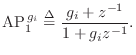
Classic Analog Phase Shifters

Setting $s=j\omega$ in Eq. $\,$ (8.19) gives the frequency response of the analog-phaser transfer function to be

$\displaystyle H_a(j\omega) \eqsp \frac{j\omega-\omega_b}{j\omega+\omega_b},$

where the `

' subscript denotes ``analog'' as opposed to ``digital''. The phase response is readily found to be

$\displaystyle \Theta_a(\omega) \eqsp \pi - 2\tan^{-1}\left(\frac{\omega}{\omega_b}\right).$

Note that the phase is always $\pi$ at dc ( $\omega=0$ ), meaning each allpass section inverts at dc. Also, at $\omega=\infty$ (remember we're talking about analog here), we get a phase of zero. In between, the phase falls from $\pi$ to 0 as frequency goes from 0 to $\infty$ . In particular, at $\omega=\omega_b$ , the phase has fallen exactly half way, to $\pi /2$ . We will call $\omega=\omega_b$ the break frequency of the allpass section.^9.23

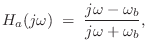
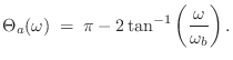
Figure 8.24a shows the phase responses of four first-order analog allpass filters with $\omega_b$ set to $2\pi[100,200,400,800]$ . Figure 8.24b shows the resulting normalized amplitude response for the phaser, for (unity feedfoward gain). The amplitude response has also been normalized by dividing by 2 so that the maximum gain is 1. Since there is an even number (four) of allpass sections, the gain at dc is . Put another way, the initial phase of each allpass section at dc is $\pi$ , so that the total allpass-chain phase at dc is $4\pi$ . As frequency increases, the phase of the allpass chain decreases. When it comes down to $3\pi$ , the net effect is a sign inversion by the allpass chain, and the phaser has a notch. There will be another notch when the phase falls down to $\pi$ . Thus, four first-order allpass sections give two notches. For each notch in the desired response we must add two new first-order allpass sections.

**Figure 8.24:** (a) Phase responses of first-order analog allpass sections with break frequencies at 100, 200, 400, and 800 Hz. (b) Corresponding phaser amplitude response.
$\includegraphics[width=\twidth]{eps/phaser1a}$

From Fig.8.24b, we observe that the first notch is near Hz. This happens to be the frequency at which the first allpass pole ``breaks,'' i.e., $\omega=g_1$ . Since the phase of a first-order allpass section at its break frequency is $\pi /2$ , the sum of the other three sections must be approximately $2\pi + \pi/2$ . Equivalently, since the first section has ``given up'' $\pi /2$ radians of phase at $\omega=g_1=2\pi100$ , the other three allpass sections combined have given up $\pi /2$ radians as well (with the second section having given up more than the other two).

In practical operation, the break frequencies must change dynamically, usually periodically at some rate.

Classic Virtual Analog Phase Shifters

To create a virtual analog phaser, following closely the design of typical analog phasers, we must translate each first-order allpass to the digital domain. Working with the transfer function, we must map from plane to the plane. There are several ways to accomplish this goal [362]. However, in this case, an excellent choice is the bilinear transform (see §7.3.2), defined by

$\displaystyle s \;\leftarrow\; c\frac{z-1}{z+1} \protect$

(9.20)

where

is chosen to map one particular frequency to exactly where it belongs. In this case,

can be chosen for each section to map the break frequency of the section to exactly where it belongs on the digital frequency axis. The relation between analog frequency $\omega_a$ and digital frequency $\omega_d$ follows immediately from Eq. $\,$ (8.20) as

$\begin{eqnarray*} j\omega_a &=& c\frac{e^{j\omega_d T}-1}{e^{j\omega_d T}+1} \eq... ...\sin(\omega_dT/2)}{\cos(\omega_dT/2)} \eqsp jc\tan(\omega_dT/2). \end{eqnarray*}$

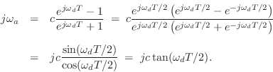
Thus, given a particular desired break-frequency $\omega_a=\omega_d=\omega_b$ , we can set

$\displaystyle c \eqsp \omega_b\cot\left(\frac{\omega_bT}{2}\right).$

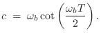
Recall from Eq. $\,$ (8.19) that the transfer function of the first-order analog allpass filter is given by

$\displaystyle H_a(s) \eqsp \frac{s-\omega_b}{s+\omega_b}$

where $\omega_b$ is the break frequency. Applying the general bilinear transformation Eq. $\,$ (8.20) gives

$\displaystyle H_d(z) \eqsp H_a\left(c\frac{1-z^{-1}}{1+z^{-1}}\right) \eqsp \f... ...1-z^{-1}}{1+z^{-1}}\right) + \omega_b}\\ \eqsp \frac{p_d-z^{-1}}{1-p_dz^{-1}}$

where we have denoted the pole of the digital allpass by

$\displaystyle p_d\isdefs \frac{c-\omega_b}{c+\omega_b} \eqsp \frac{1-\tan(\ome... ...T/2)} \;\approx\; \frac{1-\omega_bT/2}{1+\omega_bT/2} \;\approx\; 1-\omega_bT.$

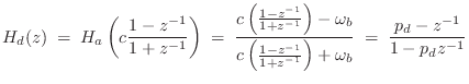
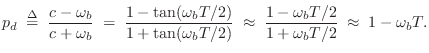
Figure 8.25 shows the digital phaser response curves corresponding to the analog response curves in Fig.8.24. While the break frequencies are preserved by construction, the notches have moved slightly, although this is not visible from the plots. An overlay of the total phase of the analog and digital allpass chains is shown in Fig.8.26. We see that the phase responses of the analog and digital alpass chains diverge visibly only above 9 kHz. The analog phase response approaches zero in the limit as $\omega_a\to\infty$ , while the digital phase response reaches zero at half the sampling rate, kHz in this case. This is a good example of when the bilinear transform performs very well.

**Figure 8.25:** (a) Phase responses of first-order digital allpass sections with break frequencies at 100, 200, 400, and 800 Hz, with the sampling rate set to 20,000 Hz. (b) Corresponding phaser amplitude response.
$\includegraphics[width=\twidth]{eps/phaser1d}$

**Figure 8.26:** Phase response of four first-order allpass sections in series -- analog and digital cases overlaid.
$\includegraphics[width=\twidth]{eps/phaser1ad}$

In general, the bilinear transform works well to digitize feedforward analog structures in which the high-frequency warping is acceptable. When frequency warping is excessive, it can be alleviated by the use of oversampling; for example, the slight visible deviation in Fig.8.26 below 10 kHz can be largely eliminated by increasing the sampling rate by 15% or so. See the case of digitizing the Moog VCF for an example in which the presence of feedback in the analog circuit leads to a delay-free loop in the digitized system [479,477].

Phasing with 2nd-Order Allpass Filters

The allpass structure proposed in [429] provides a convenient means for generating nonuniformly spaced notches that are independently controllable to a high degree. An advantage of the allpass approach even in the case of uniformly spaced notches (which we call flanging, as introduced in §5.3) is that no interpolating delay line is needed.

**Figure 8.27:** Structure of a phaser based on four second-order allpass filters.
$\includegraphics[width=4.2in]{eps/allpassphaser}$

The architecture of the phaser based on second-order allpasses is shown in Fig.8.27. It is identical to that in Fig.8.23 with each first-order allpass being replaced by a second-order allpass. I.e., replace $\hbox{AP}_{1}^{\,g_i}$ in Fig.8.23 by $\hbox{AP}_{2}^{\,g_i}$ , for , to get Fig.8.27. The phaser will have a notch wherever the phase of the allpass chain is at $\pi$ (180 degrees). It can be shown that these frequencies occur very close to the resonant frequencies of the allpass chain [429]. It is therefore convenient to use a single conjugate pole pair in each allpass section, i.e., use second-order allpass sections of the form

$\displaystyle H(z) \eqsp \frac{a_2 + a_1 z^{-1} + z^{-2}}{1 + a_1 z^{-1} + a_2 z^{-2}}$

where

$\begin{eqnarray*} a_1 &=& -2R\cos(\theta)\\ a_2 &=& R^2 \end{eqnarray*}$

and is the radius of each pole in the complex-conjugate pole pair, and pole angles are $\pm\theta$ . The pole angle can be interpreted as $\theta=\omega_c T$ where $\omega_c$ is the resonant frequency and is the sampling interval.

Phaser Notch Parameters

To move just one notch, the tuning of the pole-pair in the corresponding section is all that needs to be changed. Note that tuning affects only one coefficient in the second-order allpass structure. (Although the coefficient appears twice in the transfer function, it only needs to be used once per sample in a slightly modified direct-form implementation [449].)

The depth of the notches can be varied together by changing the gain of the feedforward path.

The bandwidth of individual notches is mostly controlled by the distance of the associated pole-pair from the unit circle. So to widen the notch associated with a particular allpass section, one may increase the ``damping'' of that section.

Finally, since the gain of the allpass string is unity (by definition of allpass filters), the gain of the entire structure is strictly bounded between 0 and 2. This property allows arbitrary notch controls to be applied without fear of the overall gain becoming ill-behaved.

Phaser Notch Distribution

As mentioned above, it is desirable to avoid exact harmonic spacing of the notches, but what is the ideal non-uniform spacing? One possibility is to space the notches according to the critical bands of hearing, since essentially this gives a uniform notch density with respect to ``place'' along the basilar membrane in the ear. There is no need to follow closely the critical-band structure, so that simple exponential spacing may be considered sufficiently perceptually uniform (corresponding to uniform spacing on a log frequency scale). Due to the immediacy of the relation between notch characteristics and the filter coefficients, the notches can easily be placed under musically meaningful control.

Next Section:
Virtual Musical Instruments
Previous Section:
Lumped Models

Transfer Function Models

Sampling the Impulse Response

Impulse Invariant Method

Relation to Finite Difference Approximation

Pole Mapping with Optimal Zeros

Modal Expansion

State Space Approach to Modal Expansions

Delay Loop Expansion

Frequency-Response Matching Using Digital Filter Design Methods

Ideal Differentiator (Spring Admittance)

Digital Filter Design Overview

Digital Differentiator Design

Fitting Filters to Measured Amplitude Responses

Converting the Desired Amplitude Response to Minimum Phase

Further Reading on Digital Filter Design

Body-Model Factoring

Extracting Parametric Resonators from a Nonparametric Impulse Response

Mode Extraction Techniques

Matlab Code for Inverse Filtering

Approximating Shortened Excitations as Noise

Body Factoring Example

Virtual Analog Example: Phasing

Phasing with First-Order Allpass Filters

Classic Analog Phase Shifters

Classic Virtual Analog Phase Shifters

Phasing with 2nd-Order Allpass Filters

Sign in

You might also like...

About this Book

Physical Audio Signal Processing

Blogs - Hall of Fame

Free PDF Downloads

Quick Links

About DSPRelated.com

Social Networks

The Related Media Group

Frequency-Response Matching Using
Digital Filter Design Methods