Search Physical Audio Signal Processing
Book Index | Global Index
Would you like to be notified by email when Julius Orion Smith III publishes a new entry into his blog?
Trapezoidal Rule
The trapezoidal rule is defined by
 |
(8.12) |
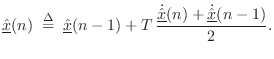
Thus, the trapezoidal rule is driven by the
average of the
derivative estimates at times

and

. The method is
implicit in either forward or reverse time.
The trapezoidal rule gets its name from the fact that it approximates
an integral by summing the areas of trapezoids. This can be seen by writing
Eq.
(7.12) as
Imagine a plot of

versus

, and connect the samples
with linear segments to form a sequence of trapezoids whose areas must
be summed to yield an approximation to

. Then the integral
at time

,

, is given by the integral at time

,

, plus the area of the next rectangle,

, plus the area of the new triangular piece atop
the new rectangle,
![$ T\,[\dot{\underline{\hat{x}}}(n) - \dot{\underline{\hat{x}}}(n-1)]/2$](http://www.dsprelated.com/josimages_new/pasp/img1708.png)
. In
other words, the integral at time

equals the integral at time

plus the area of the next trapezoid in the sum.
An interesting fact about the trapezoidal rule is that it is
equivalent to the bilinear transform in the linear,
time-invariant case. Carrying Eq.
(7.12) to the frequency domain
gives
Previous: Backward Euler MethodNext: Newton's Method of Nonlinear Minimization
About the Author: Julius Orion Smith III
Julius Smith's background is in electrical engineering (BS Rice 1975, PhD Stanford 1983). He is presently Professor of Music and Associate Professor (by courtesy) of Electrical Engineering at
Stanford's Center for Computer Research in Music and Acoustics (CCRMA), teaching courses and pursuing research related to signal processing applied to music and audio systems. See
http://ccrma.stanford.edu/~jos/ for details.