


Vector Formulation
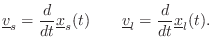
Denote the sound-source velocity by
![]() where
where
![]() is time. Similarly,
let
is time. Similarly,
let
![]() denote the velocity of the listener, if any. The
position of source and listener are denoted
denote the velocity of the listener, if any. The
position of source and listener are denoted
![]() and
and
![]() , respectively, where
, respectively, where
![]() is 3D
position. We have velocity related to position by
is 3D
position. We have velocity related to position by
Consider a Fourier component of the source at frequency
The Doppler effect depends only on velocity components along the line
connecting the source and listener [349, p. 453]. We may
therefore orthogonally project the source and listener
velocities onto the vector
![]() pointing from the source
to the listener. (See Fig.5.8 for a specific example.)
pointing from the source
to the listener. (See Fig.5.8 for a specific example.)
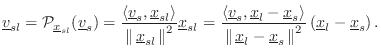
The orthogonal projection of a vector
![]() onto a vector
onto a vector
![]() is given by [451]
is given by [451]

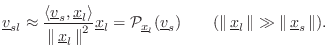
In the far field (listener far away), Eq.
Next Section:
Doppler Simulation via Delay Lines
Previous Section:
Summary of Flanging


