


Vector Wavenumber
Mathematically, a sinusoidal plane wave, as in Fig.B.9 or Fig.B.10, can be written as
where p(t,x) is the pressure at time
![$\displaystyle \underline{k}\eqsp \left[\begin{array}{c} k_x \\ [2pt] k_y \\ [2p...
... \cos{\beta} \\ [2pt] \cos{\gamma}\end{array}\right] \isdefs k\,\underline{u},
$](http://www.dsprelated.com/josimages_new/pasp/img3153.png)
-
 (unit) vector of direction cosines
-
 (scalar) wavenumber along travel
direction
(scalar) wavenumber along travel
direction
- wavenumber along the travel direction in its magnitude

- travel direction in its orientation

To see that the vector wavenumber
![]() has the claimed
properties, consider that the orthogonal projection of any
vector
has the claimed
properties, consider that the orthogonal projection of any
vector
![]() onto a vector collinear with
onto a vector collinear with
![]() is given by
is given by
![]() [451].B.35Thus,
[451].B.35Thus,
![]() is the component of
is the component of
![]() lying along the
direction of wave propagation indicated by
lying along the
direction of wave propagation indicated by
![]() . The norm of this
component is
. The norm of this
component is
![]() , since
, since
![]() is
unit-norm by construction. More generally,
is
unit-norm by construction. More generally,
![]() is the
signed length (in meters) of the component of
is the
signed length (in meters) of the component of
![]() along
along
![]() .
This length times wavenumber
.
This length times wavenumber ![]() gives the spatial phase advance along
the wave, or,
gives the spatial phase advance along
the wave, or,
![]() .
.
For another point of view, consider the plane wave
![]() ,
which is the varying portion of the general plane-wave of
Eq.
,
which is the varying portion of the general plane-wave of
Eq.![]() (B.48) at time
(B.48) at time ![]() , with unit amplitude
, with unit amplitude ![]() and zero phase
and zero phase
![]() . The spatial phase of this plane wave is given by
. The spatial phase of this plane wave is given by
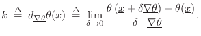
As we know from elementary vector calculus, the direction of maximum
phase advance is given by the gradient of the phase
![]() :
:
![$\displaystyle \underline{\nabla }\theta(\underline{x}) \isdefs
\left[\begin{ar...
...rray}{c} k_x \\ [2pt] k_y \\ [2pt] k_z\end{array}\right] \isdefs \underline{k}
$](http://www.dsprelated.com/josimages_new/pasp/img3172.png)
Since the wavenumber ![]() is the spatial frequency (in radians per
meter) along the direction of travel, we should be able to compute it
as the directional derivative of
is the spatial frequency (in radians per
meter) along the direction of travel, we should be able to compute it
as the directional derivative of
![]() along
along
![]() ,
i.e.,
,
i.e.,
Scattering of plane waves is discussed in §C.8.1.
Next Section:
Solving the 2D Wave Equation
Previous Section:
Plane Waves in Air


