Wave Digital Filters

The idea of wave digital filters is to digitize RLC circuits (and certain more general systems) as follows:

1. Determine the ODEs describing the system (PDEs also workable).

2. Express all physical quantities (such as force and velocity) in terms of traveling-wave components. The traveling wave components are called wave variables. For example, the force on a mass is decomposed as 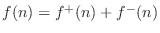, where is regarded as a traveling wave propagating toward the mass, while is seen as the traveling component propagating away from the mass. A ``traveling wave'' view of force mediation (at the speed of light) is actually much closer to underlying physical reality than any instantaneous model.

3. Next, digitize the resulting traveling-wave system using the bilinear transform (§7.3.2,[449, p. 386]). The bilinear transform is equivalent in the time domain to the trapezoidal rule for numerical integration (§7.3.2).

4. Connect elementary units together by means of -port scattering junctions. There are two basic types of scattering junction, one for parallel, and one for series connection. The theory of scattering junctions is introduced in the digital waveguide context (§C.8).

A more detailed introduction to WDFs is provided in Appendix F. In particular, the force-driven mass is considered in §F.3.4, and its wave digital model is shown in Fig.1.12.

We will not make much use of WDFs in this book, preferring instead more prosaic finite-difference models for simplicity. However, we will utilize closely related concepts in the digital waveguide modeling context (Chapter 6).

---

Previous: Impedance Networks
Next: Digital Waveguide Modeling Elements

Order a Hardcopy of Physical Audio Signal Processing

---

About the Author: Julius Orion Smith III
Julius Smith's background is in electrical engineering (BS Rice 1975, PhD Stanford 1983). He is presently Professor of Music and Associate Professor (by courtesy) of Electrical Engineering at Stanford's Center for Computer Research in Music and Acoustics (CCRMA), teaching courses and pursuing research related to signal processing applied to music and audio systems. See http://ccrma.stanford.edu/~jos/ for details.