Waveguide Transformers and Gyrators

Free Books Physical Audio Signal Processing

The ideal transformer, depicted in Fig. C.37 a, is a lossless two-port electric circuit element which scales up voltage by a constant [110,35]. In other words, the voltage at port 2 is always times the voltage at port 1. Since power is voltage times current, the current at port 2 must be times the current at port 1 in order for the transformer to be lossless. The scaling constant is called the turns ratio because transformers are built by coiling wire around two sides of a magnetically permeable torus, and the number of winds around the port 2 side divided by the winding count on the port 1 side gives the voltage stepping constant .

**Figure C.37:** a) Two-port description of the ideal transformer with ``turns ratio'' . b) Corresponding wave digital transformer.
$\includegraphics[width=\twidth]{eps/lTransformer}$

In the case of mechanical circuits, the two-port transformer relations appear as

$\begin{eqnarray*} F_2(s) &=& g F_1(s) \\ [5pt] V_2(s) &=& \frac{1}{g} V_1(s) \end{eqnarray*}$

where and denote force and velocity, respectively. We now convert these transformer describing equations to the wave variable formulation. Let and denote the wave impedances on the port 1 and port 2 sides, respectively, and define velocity as positive into the transformer. Then

$\begin{eqnarray*} f^{{+}}_1(t) &=& \frac{f_1(t) + R_1 v_1(t)}{2} \\ f^{{-}}_1(t... ...2(t)}{2} \\ &=& \frac{1}{g} \frac{f_2(t) + R_1 g^2 v_2(t)}{2}. \end{eqnarray*}$

Similarly,

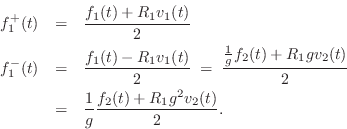
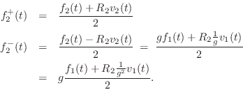
$\begin{eqnarray*} f^{{+}}_2(t) &=& \frac{f_2(t) + R_2 v_2(t)}{2} \\ f^{{-}}_2(t... ...1(t)}{2} \\ &=& g \frac{f_1(t) + R_2 \frac{1}{g^2} v_1(t)}{2}. \end{eqnarray*}$

We see that choosing

$\displaystyle g^2 = \frac{R_2}{R_1}$

eliminates the scattering terms and gives the simple relations

$\begin{eqnarray*} f^{{-}}_2(t) &=& g f^{{+}}_1(t)\\ [5pt] f^{{-}}_1(t) &=& \frac{1}{g}f^{{+}}_2(t). \end{eqnarray*}$

The corresponding wave flow diagram is shown in Fig. C.37 b.

Thus, a transformer with a voltage gain corresponds to simply changing the wave impedance from to , where $g=\sqrt{R_2/R_1}$ . Note that the transformer implements a change in wave impedance without scattering as occurs in physical impedance steps (§C.8).

Gyrators

Another way to define the ideal waveguide transformer is to ask for a two-port element that joins two waveguide sections of differing wave impedance in such a way that signal power is preserved and no scattering occurs. From Ohm's Law for traveling waves (Eq. $\,$ (6.6)), and from the definition of power waves (§C.7.5), we see that to bridge an impedance discontinuity between $R_{i-1}$ and with no power change and no scattering requires the relations

$\displaystyle \frac{[f^{{+}}_i]^2}{R_i} = \frac{[f^{{+}}_{i-1}]^2}{R_{i-1}}, \qquad\qquad \frac{[f^{{-}}_i]^2}{R_i} = \frac{[f^{{-}}_{i-1}]^2}{R_{i-1}}.$

Therefore, the junction equations for a transformer can be chosen as

$\displaystyle f^{{+}}_i= g_i\, f^{{+}}_{i-1}\qquad\qquad f^{{-}}_{i-1}= g_i^{-1}\, f^{{-}}_i \protect$

(C.125)

where

$\displaystyle g_i \isdef \pm\sqrt{\frac{R_i}{R_{i-1}}} \protect$

(C.126)

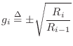
Choosing the negative square root for $g_i^{-1}$ gives a gyrator [35]. Gyrators are often used in electronic circuits to replace inductors with capacitors. The gyrator can be interpreted as a transformer in cascade with a dualizer [433]. A dualizer converts one from wave variable type (such as force) to the other (such as velocity) in the waveguide.

The dualizer is readily derived from Ohm's Law for traveling waves:

$\begin{eqnarray*} f^{{+}}\eqsp Rv^{+}, \qquad f^{{-}}\eqsp -Rv^{-}\\ [5pt] \Lon... ...i\eqsp Rv^{+}_{i-1}, \qquad v^{-}_{i-1} \eqsp -R^{-1} f^{{-}}_i \end{eqnarray*}$

In this case, velocity waves in section are converted to force waves in section , and vice versa (all at wave impedance ). The wave impedance can be changed as well by cascading a transformer with the dualizer, which changes to $R\sqrt{R_i/R}=\sqrt{RR_i}$ (where we assume $R=R_{i-1}$ ). Finally, the velocity waves in section can be scaled to equal their corresponding force waves by introducing a transformer $g=\sqrt{1/R}$ on the left, which then coincides Eq. $\,$ (C.126) (but with a minus sign in the second equation).